4.5
Solving Absolute Value Equations
and Inequalities Graphically
4.5
OBJECTIVES
1. Draw the graph of an absolute value function
2. Solve an absolute value equation graphically
3. Solve an absolute value inequality graphically
NOTE Graph the function
y x as
Equations may contain absolute value notation in their statements. In this section, we will
look at graphically solving statements that include absolute values.
To look at a graphical approach to solving, we must first look at the graph of an absolute
value function. We will start by looking at the graph of the function f(x) x. All other
graphs of absolute value functions are variations of this graph.
The graph can be found using a graphing calculator (most graphing calculators use
abs to represent the absolute value). We will develop the graph from a table of values.
Y1 abs(x)
x
3
2
1
0
1
2
f(x) x
3
2
1
0
1
2
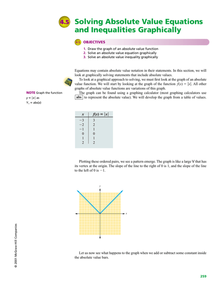
Plotting these ordered pairs, we see a pattern emerge. The graph is like a large V that has
its vertex at the origin. The slope of the line to the right of 0 is 1, and the slope of the line
to the left of 0 is 1.
y
© 2001 McGraw-Hill Companies
x
Let us now see what happens to the graph when we add or subtract some constant inside
the absolute value bars.
259
260
CHAPTER 4
GRAPHS OF LINEAR EQUATIONS AND FUNCTIONS
Example 1
Graphing an Absolute Value Function
Graph each function.
would be entered as
Y1 abs(x 3)
(a) f(x) x 3
Again, we start with a table of values.
x
2
1
0
1
2
3
4
5
f(x)
5
4
3
2
1
0
1
2
Then, we plot the points associated with the set of ordered pairs.
y
x
The graph of the function f(x) x 3 is the same shape as the graph of the function
f(x) x; it has just shifted to the right 3 units.
(b) f(x) x 1
We begin with a table of values.
x
2
1
0
1
2
3
f(x)
1
0
1
2
3
4
© 2001 McGraw-Hill Companies
NOTE f(x) x 3
SOLVING ABSOLUTE VALUE EQUATIONS AND INEQUALITIES GRAPHICALLY
SECTION 4.5
261
Then we graph.
y
x
Note that the graph of f(x) x 1 is the same shape as the graph of the function
f(x) x, except that it is shifted 1 unit to the left.
CHECK YOURSELF 1
Graph each function.
(a) f(x) x 2
(b) f(x) x 3
We can summarize what we have discovered about the horizontal shift of the graph of an
absolute value function.
Rules and Properties:
Graphing Absolute Value Functions
The graph of the function f(x) x a will be the same shape as the graph of
f(x) x except that the graph will be shifted a units
NOTE If a is negative, x a
to the right if a is positive
to the left if a is negative
will be x plus some positive
number. For example, if a 2,
x a x (2) x 2
© 2001 McGraw-Hill Companies
We will now use these methods to solve equations that contain an absolute value expression.
Example 2
Solving an Absolute Value Equation Graphically
NOTE Algebraically
x 3 4
x 3 4 or x 3 4
x 7 or x 1
Graphically, find the solution set for the equation.
x 3 4
CHAPTER 4
GRAPHS OF LINEAR EQUATIONS AND FUNCTIONS
We graph the function associated with each side of the equation.
f(x) x 3
and
g(x) 4
y
f
g
x
Then, we draw a vertical line through each of the intersection points.
y
f
g
x
We ask the question,
“For what values of x
do f and g coincide?”
Looking at the x values of the two vertical lines, we find the solutions to the original
equation. There are two x values that make the statement true: 1 and 7. The solution set
is 1, 7.
CHECK YOURSELF 2
Graphically find the solution set for the equation.
x 2 3
Example 3 demonstrates a graphical approach to solving an absolute value inequality.
Example 3
Solving an Absolute Value Inequality Graphically
Graphically solve
x 6
As we did in previous sections, we begin by letting each side of the inequality represent
a function. Here
f(x) x
and
g(x) 6
© 2001 McGraw-Hill Companies
262
SOLVING ABSOLUTE VALUE EQUATIONS AND INEQUALITIES GRAPHICALLY
SECTION 4.5
263
Now we graph both functions on the same set of axes.
y
f
g
x
We now ask the question,
“For what values of x is f
below g?”
We next draw a dotted line (equality is not included) through the points of intersection
of the two graphs.
y
f
g
x
The solution set is any value of x for which the graph of f(x) is below the graph of g(x).
y
f
g
x
© 2001 McGraw-Hill Companies
The solution
set
In set notation, we write x 6 x 6.
CHECK YOURSELF 3
Graphically solve the inequality
x 3
CHAPTER 4
GRAPHS OF LINEAR EQUATIONS AND FUNCTIONS
CHECK YOURSELF ANSWERS
1. (a)
f(x) x 2
y
x
(b)
y
f(x) x 3
x
2.
3.
y
x
y
x
{1, 5}
xx 3 or x 3
© 2001 McGraw-Hill Companies
264
Name
4.5
Exercises
Section
Date
In exercises 1 to 6, graph each function.
1. f(x) x 3
2. f(x) x 2
ANSWERS
y
y
1.
2.
3.
x
4.
5.
3. f(x) x 3
4. f(x) x 4
y
6.
y
7.
8.
x
5. f(x) x (3)
x
6. f(x) x (5)
y
y
x
x
In exercises 7 to 12, solve the equations graphically.
© 2001 McGraw-Hill Companies
7. x 3
8. x 5
y
y
x
x
265
ANSWERS
9.
9. x 2 10.
7
2
10. x 5 3
y
y
11.
12.
x
13.
x
14.
15.
16.
11. x 2 4
12. x 4 2
y
y
x
x
In exercises 13 to 16, determine the function represented by each graph.
14.
y
y
x
15.
x
16.
y
x
266
y
x
© 2001 McGraw-Hill Companies
13.
ANSWERS
17.
In exercises 17 to 28, solve each inequality graphically.
17. x 4
18.
18. x 6
19.
y
y
20.
21.
x
x
22.
23.
24.
19. x 5
20. x 2
y
y
x
21. x 3 4
x
22. x 1 5
y
y
x
23. x 2 5
24. x 2 4
y
© 2001 McGraw-Hill Companies
x
y
x
x
267
ANSWERS
25.
25. x 1 5
26.
26. x 4 1
y
y
27.
28.
x
x
29.
27. x 2 2
28. x 4 1
y
y
x
x
29. Assessing Piston Design. Combustion engines get their power from the force
1. Write an absolute value statement about the diameter, dc , of the cylinder.
2. If the diameter of the piston is to be 7.59 cm with a tolerance of 0.1 mm, write an
absolute value statement about the diameter, dp , of the piston.
3. Investigate all the possible ways these two parts will fit together. If the two parts
have to be within 0.1 mm of each other for the engine to run well, is there a
problem with the way the parts may be paired together? Write your answer and use
a graph to explain.
268
© 2001 McGraw-Hill Companies
exerted by burning fuel on a piston inside a chamber. The piston is forced down out
of the cylinder by the force of a small explosion caused by burning fuel mixed with
air. The piston in turn moves a piston rod, which transfers the motion to the work of
the engine. The rod is attached to a flywheel, which pushes the piston back into the
cylinder to begin the process all over. Cars usually have four to eight of these
cylinders and pistons. It is crucial that the piston and the cylinder fit well together,
with just a thin film of oil separating the sides of the piston and the sides of the
cylinder. When these are manufactured, the measurements for each part must be
accurate. But, there is always some error. How much error is a matter for the
engineers to set and for the quality control department to check.
Suppose the diameter of the cylinder is meant to be 7.6 cm, and the engineer
specifies that this part must be manufactured to within 0.1 mm of that measurement.
This figure is called the tolerance. As parts come off the assembly line, someone in
quality control takes samples and measures the cylinders and the pistons. Given this
information, complete the following.
4. Accuracy in machining the parts is expensive, so the tolerance should be close
enough to make sure the engine runs correctly, but not so close that the cost is
prohibitive. If you think a tolerance of 0.1 mm is too large, find another that you
think would work better. If it is too small, how much can it be enlarged and still
have the engine run according to design? (That is, so dc dp 0.1 mm.) Write
the tolerance using absolute value signs. Explain your reasoning if you think a
tolerance of 0.1 mm is not workable.
5. After you have decided on the appropriate tolerance for these parts, think
about the quality control engineer’s job. Hazard a few educated opinions to
answer these questions: How many parts should be pulled off the line and
measured? How often? How many parts can reasonably be expected to be
outside the expected tolerance before the whole line is shut down and the tools
corrected?
Answers
y
1.
3.
y
x
5.
x
7.
y
f(x) x
y
g(x) 3
x
3
3
x
{3, 3}
© 2001 McGraw-Hill Companies
9.
f(x) x 2
11.
y
g(x) 3
2
11
2
x
{32 , 112 }
f(x) x 2
y
g(x) 4
7
2
6
2
x
{6, 2}
269
13. f(x) x 2
17.
15. f(x) x 2
19.
y
f(x) x
f(x) x
y
g(x) 5
g(x) 4
x
x
{x 4 x 4}
21.
f(x) x 3
{xx 5 or x 5}
23.
y
f(x) x 2
y
g(x) 5
g(x) 4
x
x
1
7
{xx 3 or x 7}
{x 1 x 7}
25.
y
f(x) x 1
27.
y
f(x) x 2
g(x) 5
x
x
g(x) 2
{x 6 x 4}
All real numbers
© 2001 McGraw-Hill Companies
29.
270