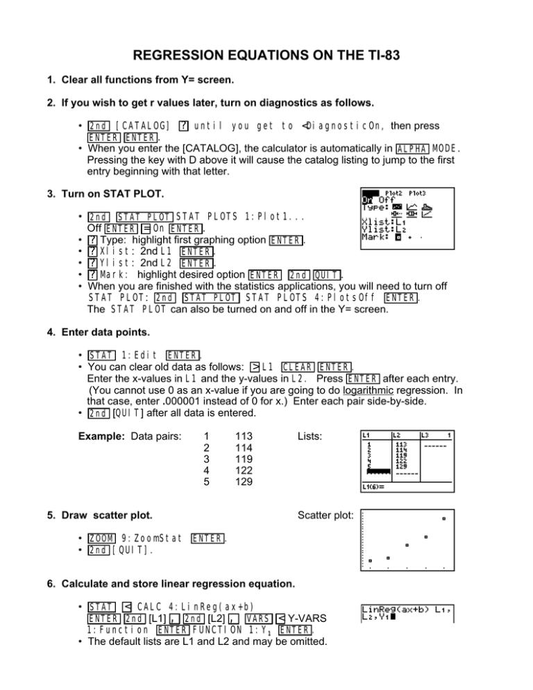
REGRESSION EQUATIONS ON THE TI-83
1. Clear all functions from Y= screen.
2. If you wish to get r values later, turn on diagnostics as follows.
• 2nd [CATALOG] ? until you get to <DiagnosticOn, then press
ENTER ENTER .
• When you enter the [CATALOG], the calculator is automatically in ALPHA MODE.
Pressing the key with D above it will cause the catalog listing to jump to the first
entry beginning with that letter.
3. Turn on STAT PLOT.
• 2nd STAT PLOT STAT PLOTS 1:Plot1...
Off ENTER = On ENTER .
• ? Type: highlight first graphing option ENTER .
• ? Xlist: 2nd L1 ENTER .
• ? Ylist: 2nd L2 ENTER .
• ? Mark: highlight desired option ENTER 2nd QUIT .
• When you are finished with the statistics applications, you will need to turn off
STAT PLOT: 2nd STAT PLOT STAT PLOTS 4:PlotsOff ENTER .
The STAT PLOT can also be turned on and off in the Y= screen.
4. Enter data points.
• STAT 1:Edit ENTER .
• You can clear old data as follows: > L1 CLEAR ENTER .
Enter the x-values in L1 and the y-values in L2. Press ENTER after each entry.
(You cannot use 0 as an x-value if you are going to do logarithmic regression. In
that case, enter .000001 instead of 0 for x.) Enter each pair side-by-side.
• 2nd [QUIT] after all data is entered.
Example: Data pairs:
1
2
3
4
5
113
114
119
122
129
5. Draw scatter plot.
Lists:
Scatter plot:
• ZOOM 9:ZoomStat ENTER .
• 2nd [QUIT].
6. Calculate and store linear regression equation.
• STAT
< CALC 4:LinReg(ax+b)
ENTER 2nd [L1] , 2nd [L2] , VARS < Y-VARS
1:Function ENTER FUNCTION 1:Y1 ENTER .
• The default lists are L1 and L2 and may be omitted.
• The coefficients and r value are displayed on the home
screen.
• The regression equation is stored in Y1=.
7. Superimpose regression line on scatterplot.
• ZOOM ZOOM 9:ZoomStat ENTER .
8. The correlation coefficient r.
• The correlation coefficient r is a number between –1 and +1 that indicates the
closeness of the fit of the regression line. The closer |r| is to 1, the better the fit.
This line is a good fit, but there may be another type of regression that is better.
9. Using the regression equation to predict other y-values.
• Example: To find y when x = 10: VARS < Y-VARS 1:Function ENTER
FUNCTION 1:Y1 ENTER ( 1 0 ) ENTER
• You could also store 10 as X and then evaluate Y1.
• You could also use the graph and the 2nd CALC CALCULATE 1:value option.
10. Clearing an entire list of old data.
• There are several methods for clearing old data, but one of the easiest is: STAT
1:Edit,use the up arrow > highlight the name of the list you wish to clear, then
press CLEAR ENTER
11. Calculating other types of regression models.
• Quadratic model:
y = .714x2 – .286x + 112.4
(rounded to 3 decimals)
• Cubic model:
y = .714x2 – .286x + 112.4
Isn’t that strange!!
• Quartic model:
y = .5x4 – 6x3 + 25.5x2
– 41x + 134
• Natural logarithmic
model:
y = 9.206ln x + 110.585
• Exponential model:
y = 107.933*(1.034x)
• Power regression model:
y = 110.799*x.077
Regression Equations on the TI-83
Judy Ahrens
Pellissippi State Technical Community College
January 30, 1999