Polyphase Decomposition
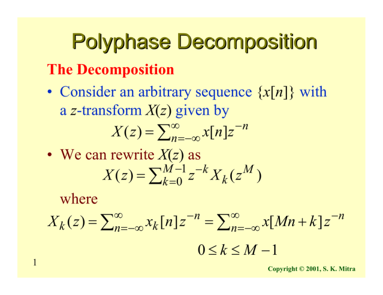
The Decomposition
• Consider an arbitrary sequence {x[n]} with
a z-transform X(z) given by
∞
X ( z ) = ∑n = −∞ x[n]z − n
• We can rewrite X(z) as
M −1 − k
M
X ( z ) = ∑ k =0 z X k ( z )
where
∞
∞
−n
−n
X k ( z ) = ∑n = −∞ xk [n] z = ∑n = −∞ x[Mn + k ] z
0 ≤ k ≤ M −1
1
Copyright © 2001, S. K. Mitra
Polyphase Decomposition
• The subsequences {xk [n]} are called the
polyphase components of the parent
sequence {x[n]}
• The functions X k (z ), given by the
z-transforms of {xk [n]}, are called the
polyphase components of X(z)
2
Copyright © 2001, S. K. Mitra
Polyphase Decomposition
• The relation between the subsequences {xk [n]}
and the original sequence {x[n]} are given
by
xk [n] = x[Mn + k ], 0 ≤ k ≤ M − 1
• In matrix form we can write
[
X ( z ) = 1 z −1 .... z −( M −1)
3
 X0(zM ) 


M
 X1.( z ) 
..


 X . ( z M )

 M −1
]
Copyright © 2001, S. K. Mitra
Polyphase Decomposition
• A multirate structural interpretation of the
polyphase decomposition is given below
4
Copyright © 2001, S. K. Mitra
Polyphase Decomposition
• The polyphase decomposition of an FIR
transfer function can be carried out by
inspection
• For example, consider a length-9 FIR
transfer function:
H ( z) =
8
∑ h[n] z
−n
n =0
5
Copyright © 2001, S. K. Mitra
Polyphase Decomposition
• Its 4-branch polyphase decomposition is
given by
4
−1
4
−2
4
−3
4
H ( z ) = E0 ( z ) + z E1( z ) + z E2 ( z ) + z E3 ( z )
where
−1
−2
E0 ( z ) = h[0] + h[4]z + h[8]z
E1( z ) = h[1] + h[5]z −1
−1
E2 ( z ) = h[2] + h[6]z
−1
E3 ( z ) = h[3] + h[7]z
6
Copyright © 2001, S. K. Mitra
Polyphase Decomposition
• The polyphase decomposition of an IIR
transfer function H(z) = P(z)/D(z) is not that
straight forward
• One way to arrive at an M-branch polyphase
decomposition of H(z) is to express it in the
form P '( z ) / D '( z M ) by multiplying P(z) and
D(z) with an appropriately chosen
polynomial and then apply an M-branch
polyphase decomposition to P '( z )
7
Copyright © 2001, S. K. Mitra
Polyphase Decomposition
• Example - Consider
1− 2 z −1
H ( z) =
−1
1+3 z
• To obtain a 2-band polyphase decomposition
we rewrite H(z) as
H ( z) =
8
(1− 2 z −1 )(1−3 z −1 )
(1+3 z −1 )(1−3 z −1 )
1−5 z −1 + 6 z − 2
=
1−9 z − 2
1+ 6 z − 2
=
1−9 z − 2
−5 z −1
+
1−9 z − 2
• Therefore,
2
−1
2
H ( z ) = E0 ( z ) + z E1( z )
where
−5
1+ 6 z −1
E0 ( z ) =
, E1( z ) =
−1
−1
1−9 z
1−9 z
Copyright © 2001, S. K. Mitra
Polyphase Decomposition
• Note: The above approach increases the
overall order and complexity of H(z)
• However, when used in certain multirate
structures, the approach may result in a
more computationally efficient structure
• An alternative more attractive approach is
discussed in the following example
9
Copyright © 2001, S. K. Mitra
Polyphase Decomposition
• Example - Consider the transfer function of
a 5-th order Butterworth lowpass filter with
a 3-dB cutoff frequency at 0.5π:
H ( z) =
0.0527864 (1+ z −1 )5
1+ 0.633436854 z − 2 + 0.0557281z − 2
• It is easy to show that H(z) can be expressed
as
−2
−2
−1 0.52786 + z  
1  0.105573 + z 
H ( z ) = 
+z 

−
2
−2 
2  1+ 0.105573 z 
 1+ 0.52786 z 
10
Copyright © 2001, S. K. Mitra
Polyphase Decomposition
• Therefore H(z) can be expressed as
2
−1
2
H ( z ) = E0 ( z ) + z E1( z )
where
11
E0 ( z ) =
−1
1  0.105573 + z 
2  1+ 0.105573 z −1 
E1( z ) =
−1
1  0.52786 + z 
2  1+ 0.52786 z −1 
Copyright © 2001, S. K. Mitra
Polyphase Decomposition
• Note: In the above polyphase decomposition,
branch transfer functions Ei (z ) are stable
allpass functions
• Moreover, the decomposition has not
increased the order of the overall transfer
function H(z)
12
Copyright © 2001, S. K. Mitra
FIR Filter Structures Based on
Polyphase Decomposition
• We shall demonstrate later that a parallel
realization of an FIR transfer function H(z)
based on the polyphase decomposition can
often result in computationally efficient
multirate structures
• Consider the M-branch Type I polyphase
decomposition of H(z):
H ( z) = ∑
13
M −1 − k
M)
z
E
z
(
k
k =0
Copyright © 2001, S. K. Mitra
FIR Filter Structures Based on
Polyphase Decomposition
• A direct realization of H(z) based on the
Type I polyphase decomposition is shown
below
14
Copyright © 2001, S. K. Mitra
FIR Filter Structures Based on
Polyphase Decomposition
• The transpose of the Type I polyphase FIR
filter structure is indicated below
15
Copyright © 2001, S. K. Mitra
FIR Filter Structures Based on
Polyphase Decomposition
• An alternative representation of the
transpose structure shown on the previous
slide is obtained using the notation
Rl ( z M ) = EM −1−l ( z M ),
0 ≤ l ≤ M −1
• Substituting the above notation in the Type
I polyphase decomposition we arrive at the
Type II polyphase decomposition:
H ( z) = ∑
16
M −1 −( M −1−l )
M)
(
z
R
z
l
l =0
Copyright © 2001, S. K. Mitra
FIR Filter Structures Based on
Polyphase Decomposition
• A direct realization of H(z) based on the
Type II polyphase decomposition is shown
below
17
Copyright © 2001, S. K. Mitra
Computationally Efficient
Decimators
• Consider first the single-stage factor-of-M
decimator structure shown below
x[n ]
H (z)
v[n]
M
y[n ]
• We realize the lowpass filter H(z) using the
Type I polyphase structure as shown on the
next slide
18
Copyright © 2001, S. K. Mitra
Computationally Efficient
Decimators
• Using the cascade equivalence #1 we arrive
at the computationally efficient decimator
structure shown below on the right
x[n]
y[n] x[n]
y[n]
v[n ]
Decimator structure based on Type I polyphase decomposition
19
Copyright © 2001, S. K. Mitra
Computationally Efficient
Decimators
• To illustrate the computational efficiency of
the modified decimator structure, assume
H(z) to be a length-N structure and the input
sampling period to be T = 1
• Now the decimator output y[n] in the
original structure is obtained by downsampling the filter output v[n] by a factor of
M
20
Copyright © 2001, S. K. Mitra
Computationally Efficient
Decimators
• It is thus necessary to compute v[n] at
n = ...,−2 M , − M , 0, M ,2 M , ...
• Computational requirements are therefore N
multiplications and ( N − 1) additions per
output sample being computed
• However, as n increases, stored signals in
the delay registers change
21
Copyright © 2001, S. K. Mitra
Computationally Efficient
Decimators
• Hence, all computations need to be
completed in one sampling period, and for
the following ( M − 1) sampling periods the
arithmetic units remain idle
• The modified decimator structure also
requires N multiplications and ( N − 1)
additions per output sample being computed
22
Copyright © 2001, S. K. Mitra
Computationally Efficient
Decimators and Interpolators
• However, here the arithmetic units are
operative at all instants of the output
sampling period which is M times that of
the input sampling period
• Similar savings are also obtained in the case
of the interpolator structure developed using
the polyphase decomposition
23
Copyright © 2001, S. K. Mitra
Computationally Efficient
Interpolators
• Figures below show the computationally
efficient interpolator structures
24
Interpolator based on
Type I polyphase decomposition
Interpolator based on
Type II polyphase decomposition
Copyright © 2001, S. K. Mitra
Computationally Efficient
Decimators and Interpolators
• More efficient interpolator and decimator
structures can be realized by exploiting the
symmetry of filter coefficients in the case of
linear-phase filters H(z)
• Consider for example the realization of a
factor-of-3 (M = 3) decimator using a
length-12 Type 1 linear-phase FIR lowpass
filter
25
Copyright © 2001, S. K. Mitra
Computationally Efficient
Decimators and Interpolators
• The corresponding transfer function is
H ( z ) = h[ 0] + h[1] z −1 + h[ 2] z − 2 + h[3] z −3 + h[ 4] z − 4 + h[5] z −5
+ h[5] z −6 + h[ 4] z −7 + h[3] z −8 + h[ 2] z −9 + h[1] z −10 + h[ 0] z −11
26
• A conventional polyphase decomposition of
H(z) yields the following subfilters:
E0 ( z ) = h[0] + h[3]z −1 + h[5]z − 2 + h[2]z −3
E1 ( z ) = h[1] + h[4]z −1 + h[4]z − 2 + h[1]z −3
E2 ( z ) = h[2] + h[5]z −1 + h[3]z − 2 + h[0]z −3
Copyright © 2001, S. K. Mitra
Computationally Efficient
Decimators and Interpolators
• Note that E1 ( z ) still has a symmetric
impulse response, whereas E0 ( z ) is the
mirror image of E2 ( z )
• These relations can be made use of in
developing a computationally efficient
realization using only 6 multipliers and 11
two-input adders as shown on the next slide
27
Copyright © 2001, S. K. Mitra
Computationally Efficient
Decimators and Interpolators
• Factor-of-3 decimator with a linear-phase
decimation filter
28
Copyright © 2001, S. K. Mitra
A Useful Identity
• The cascade multirate structure shown
below appears in a number of applications
x[n]
L
H(z)
L
y[n]
• Equivalent time-invariant digital filter
obtained by expressing H(z) in its L-term
Type I polyphase form ∑ kL=−10 z −k Ek ( z L )
is shown below
x[n]
29
E0 ( z )
y[n]
Copyright © 2001, S. K. Mitra
Arbitrary-Rate Sampling Rate
Converter
• The estimation of a discrete-time signal
value at an arbitrary time instant between a
consecutive pair of known samples can be
solved by using some type of interpolation
• In this approach an approximating
continuous-time signal is formed from a set
of known consecutive samples of the given
discrete-time signal
30
Copyright © 2001, S. K. Mitra
Arbitrary-Rate Sampling Rate
Converter
• The value of the approximating continuoustime signal is then evaluated at the desired
time instant
• This interpolation process can be directly
implemented by designing a digital
interpolation filter
31
Copyright © 2001, S. K. Mitra
Ideal Sampling Rate
Converter
• In principle, a sampling rate conversion by
an arbitrary conversion factor can be
implemented as follows
• The input digital signal is passed through an
ideal analog reconstruction lowpass filter
whose output is resampled at the desired
output rate as indicated below
32
Copyright © 2001, S. K. Mitra
Ideal Sampling Rate
Converter
• Let the impulse response of the analog
lowpass filter is denoted by g a (t )
• Then the output of the filter is given by
∞
^
xa (t ) = ∑l = −∞ x[l]g a (t − lT )
• If the analog filter is chosen to bandlimit its
output to the frequency range Fg < FT' / 2 ,
its output ^xa (t ) can then be resampled at the
rate FT'
33
Copyright © 2001, S. K. Mitra
Ideal Sampling Rate
Converter
• Since the impulse response g a (t ) of an ideal
lowpass analog filter is of infinite duration
and the samples g a (nT '−lT ) have to be
computed at each sampling instant,
implementation of the ideal bandlimited
interpolation algorithm in exact form is not
practical
• Thus, an approximation is employed in
practice
34
Copyright © 2001, S. K. Mitra
Ideal Sampling Rate
Converter
• Problem statement: Given N 2 + N1 + 1 input
signal samples, x[k], k = − N1, ..., N 2 , obtained
by sampling an analog signal xa (t ) at t = tk
= t0 + kTin , determine the sample value
xa (t0 + kTin ) = y[α ] at time instant t ' = t0 + kTin
where − N1 ≤ α ≤ N 2
• Figure on the next slide illustrates the
interpolation process by an arbitrary factor
35
Copyright © 2001, S. K. Mitra
Ideal Sampling Rate
Converter
• We describe next a commonly employed
interpolation algorithm based on a finite
weighted sum of input samples
36
Copyright © 2001, S. K. Mitra
Lagrange Interpolation
Algorithm
• Here, a polynomial approximation ^xa (t ) to
xa (t ) is defined as
^
xa (t ) =
37
N2
∑ Pk (t )x[n + k ]
k = − N1
where Pk (t ) are the Lagrange polynomials
given by
N2
 t − tk 
Pk (t ) = ∏ 
, − N1 ≤ k ≤ N 2
l = − N1  tk − tl 
l≠k
Copyright © 2001, S. K. Mitra
Lagrange Interpolation
Algorithm
• Example - Design a fractional-rate
interpolator with an interpolation factor of
3/2 using a 3rd-order polynomial
approximation with N1 = 2 and N 2 = 1
• The output y[n] of the interpolator is thus
computed using
y[n] = P− 2 (α) x[n − 2] + P−1 (α) x[n − 1]
+ P0 (α) x[n] + P1 (α) x[n + 1]
38
Copyright © 2001, S. K. Mitra
Lagrange Interpolation
Algorithm
• Here, the Lagrange polynomials are given
by
( α +1) α ( α −1) 1
P− 2 (α) =
= ( −α 3 + α )
−6
6
( α + 2) α ( α −1) 1 3
P−1 (α) =
= ( α + α 2 − 2α )
2
2
( α + 2)(α +1)(α −1)
1 3
P0 (α) =
= − ( α + 2α 2 − α − 2)
−2
2
( α + 2)(α +1) α 1 3
P1 (α) =
= (α + 3α 2 + α)
−6
6
39
Copyright © 2001, S. K. Mitra
Lagrange Interpolation
Algorithm
• Figure below shows the locations of the
samples of the input and the output for an
interpolator with a conversion factor of 3/2
• Locations of the output samples y[0], y[1],
and y[2] in the input sample domain are
marked with an arrow
↓
↓
↓
Input sample index
Output sample index
40
Copyright © 2001, S. K. Mitra
Lagrange Interpolation
Algorithm
• From the figure on the previous slide it can
be seen that the value of α for computation
of y[n], to be labeled α 0 , is 0
• Substituting this value of α in the
expressions for the Lagrange polynomial
coefficients derived earlier we get
P− 2 (α 0 ) = 0 , P−1 (α 0 ) = 0
P0 (α 0 ) = 1 , P1 (α 0 ) = 0
41
Copyright © 2001, S. K. Mitra
Lagrange Interpolation
Algorithm
• The value of α for computation of y[n+1],
to be labeled α1 , is 2/3
• Substituting this value of α in the
expressions for the Lagrange polynomial
coefficients we get
P− 2 (α1 ) = 0.0617 , P−1 (α1 ) = −0.2963
P0 (α1 ) = 0.7407 , P1 (α1 ) = 0.4938
42
Copyright © 2001, S. K. Mitra
Lagrange Interpolation
Algorithm
• The value of α for computation of y[n+2],
to be labeled α 2 , is 4/3
• Substituting this value of α in the
expressions for the Lagrange polynomial
coefficients we get
P− 2 (α 2 ) = −0.1728 , P−1 (α 2 ) = 0.7407
P0 (α 2 ) = −1.2963 , P1 (α 2 ) = 1.7284
43
Copyright © 2001, S. K. Mitra
Lagrange Interpolation
Algorithm
• Substituting the values of the Lagrange
polynomial coefficients in the interpolator
output equation for n, n+1, and n+2, and
combining the three equations into a matrix
form we arrive at
 y[ n]   P−2 (α 0 )
 P− 2 ( α1 )
y
[
n
1
]
+
=

 
 y[ n + 2]  P−2 (α 2 )
44
P−1 ( α 0 ) P0 ( α 0 ) P1 ( α 0 ) 
P−1 ( α1 ) P0 ( α1 ) P1 ( α1 ) 
P−1 ( α 2 ) P0 ( α 2 ) P1 ( α 2 ) 
 x[ n − 2]
 x[ n −1] 
 x[ n ] 
 x[ n +1] 


Copyright © 2001, S. K. Mitra
Lagrange Interpolation
Algorithm
• The input-output relation of the
interpolation filter can be compactly written
as
x[ n − 2]

y
n
[
]


x[ n −1] 

y
n
[
1
]
+
=

 H x[ n]
 x[ n +1] 
 y[ n + 2]


where H is the block coefficient matrix
45
Copyright © 2001, S. K. Mitra
Lagrange Interpolation
Algorithm
• For the factor-of-3/2 interpolator, we have
H
0
1
0 
 0
=  0.0617 −0.2963 0.7407 0.4938
 −0.1728 0.7407 −1.2963 1.7284 
• It should be evident from an examination of
↓
↓
↓
Input sample index
Output sample index
that the filter coefficients to compute
y[n+3], y[n+4], and y[n+5] are again given
by the same block matrix H
46
Copyright © 2001, S. K. Mitra
Lagrange Interpolation
Algorithm
•
The desired interpolation filter is a
time-varying filter
• A realization of the interpolator is given
below
47
Copyright © 2001, S. K. Mitra
Lagrange Interpolation
Algorithm
• Note: In practice, the overall system delay
will be 3 sample periods
• Hence, the output sample y[n] actually will
appear at the time index n+3
• A realization of the factor-of-3 interpolator
in the form of a time-varying filter is shown
on the next slide
48
Copyright © 2001, S. K. Mitra
Lagrange Interpolation
Algorithm
• The coefficients of the 5-th order timevarying FIR filter have a period of 3 and are
assigned the values indicated below
49
Copyright © 2001, S. K. Mitra
Lagrange Interpolation
Algorithm
• Substituting the expressions for the Lagrange
polynomials in the output equation we arrive
at
y[n] = α3 (− 1 x[n − 2] + 1 x[n − 1] − 1 x[n] + 1 x[n + 1])
6
2
2
6
+ α 2 ( 1 x[n − 1] − x[n] + 1 x[n + 1])
2
2
+ α( 1 x[n − 2] − x[n − 1] + 1 x[n] + 1 x[n + 1])
6
2
3
+ x[n]
50
Copyright © 2001, S. K. Mitra
Lagrange Interpolation
Algorithm
• A digital filter realization of the equation on
the previous slide leads to the Farrow
structure shown below
• In the above structure
H 0 ( z ) = − 16 z − 2 + 12 z −1 − 12 + 16 z
H1 ( z ) = 12 z −1 − 1 + 12 z
51
H 2 ( z ) = 16 z − 2 − z −1 + 12 + 13 z
Copyright © 2001, S. K. Mitra
Lagrange Interpolation
Algorithm
• In the Farrow structure only the value of a is
changed periodically with the remaining
digital filter structure kept unchanged
• Figures on the next slide show the input and
the output of the above interpolator for a
sinusoidal input of frequency of 0.05 Hz
sampled at a 1-Hz rate
52
Copyright © 2001, S. K. Mitra
Lagrange Interpolation
Algorithm
Interpolator Output
1
1
0.5
0.5
Amplitude
Amplitude
Input Sinusoidal Sequence
0
-0.5
-1
0
5
10
15
20
25
30
Time index n, sampling interval = 1 sec.
0
-0.5
-1
0
10
20
30
40
50
Time index n, sampling interval = 2/3 sec.
Error Sequence
0.1
Amplitude
0.05
0
-0.05
-0.1
53
0
10
20
30
40
50
Copyright © 2001, S. K. Mitra
Time index n, sampling interval = 2/3 sec.
Arbitrary-Rate Sampling Rate
Converter
Practical Considerations
• A direct design of a fractional-rate sampling
rate converter in most applications is not
practical
• This is due to two main reasons:
– length of the time-varying filter needed is
usually very large
– real-time computation of the corresponding
filter coefficients is nearly impossible
54
Copyright © 2001, S. K. Mitra
Arbitrary-Rate Sampling Rate
Converter
• As a result, the fractional-rate sampling rate
converter is almost realized in a hybrid form
as indicated below for the case of an
interpolator
55
• The digital sampling rate converter can be
implemented in a multistage form to reduce
the computational complexity
Copyright © 2001, S. K. Mitra