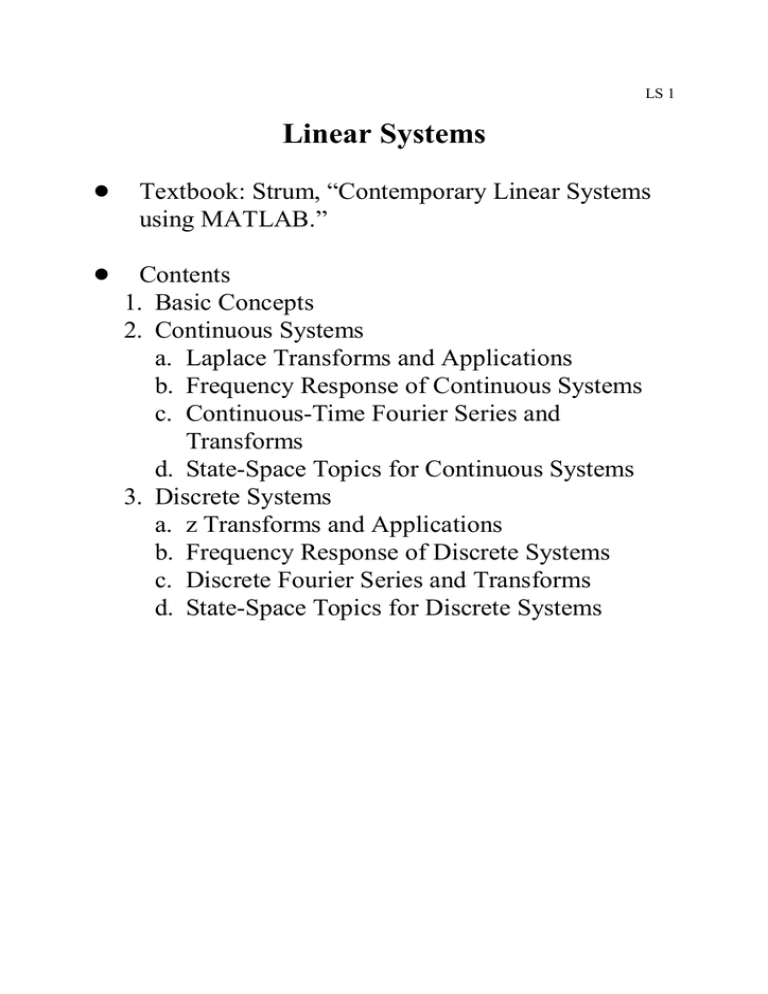
LS 1
Linear Systems
!
!
Textbook: Strum, “Contemporary Linear Systems
using MATLAB.”
Contents
1. Basic Concepts
2. Continuous Systems
a. Laplace Transforms and Applications
b. Frequency Response of Continuous Systems
c. Continuous-Time Fourier Series and
Transforms
d. State-Space Topics for Continuous Systems
3. Discrete Systems
a. z Transforms and Applications
b. Frequency Response of Discrete Systems
c. Discrete Fourier Series and Transforms
d. State-Space Topics for Discrete Systems
LS 2
Chap. 1 Basic Concepts
Continus V. S. Discrete
Continuous System
Discrete System
LS 3
Unit Impulse
1. A virtual function.
2. Any arbitrary analog signal can be decomposed by impulses.
3. The response of any analog signal can be decomposed by impulse
responses.
Properties:
(Sifting Property)
Example:
LS 4
Unit Step Function
Representing Signals
a.
b.
LS 5
Conversion between Continuous and Discrete Signals
Sampling Theorem: Let
: the maximum frequency component of the signal,
: the sampling frequency.
then
if the signal can be uniquely represented by the
samples, or the signal can fully recovered from the samples.
LS 6
Chap. 2 Continuous Systems
Basic Concept
Linearity: A system is linear if and only if it satisfies the principle of
homogeneity and additivity.
1. Homogeneity
2. Additivity
3. Homogeneity and additivity
LS 7
Time Invariance: The same input applied at different times will
produce the same output except shifted in time. That is, for arbitrary
Linear Time-Invariant Systems (LTI): Linear + time-invariant.
1. Can be analyzed by Laplace and Fourier transforms.
2. In time domain, described by linear differential equations with
constant coefficients.
3. In transform domains, described by linear algebraic equation.
Causality: Output depends on only previous inputs. That is,
depends on
only
.
LS 8
Stability: if the input is bounded, the output is also bounded
(bounded-input-bounded-output BIBO).
Problems 2.1. Discuss the properties of the following continuous
systems.
a.
. (i) Linear? (ii) Time invariant?
b.
. Causal or noncausal?
c.
Nth-Order Differential Equation Model
In general, a single-input-single-output LTI system can be modeled
by Nth-order differential equation as follows,
Example:
Initial Condition Solution of a Differential Equation
1. Find the homogeneous solution, i.e.
LS 9
Let
, substitute this to the above equation. Then,
which is a polynomial called characteristic equation.
Let
be the roots of the characteristic equation, then
Note: if stable, the real parts of the roots must be negative.
The initial condition solution is in the form
where
are unknown coefficients to be determined by the
initial conditions
.
Problem 2.2
Let
a. Find the system’s characteristic
equation.
b. Find the root.
c. Is the system stable?
d. Find the general form of the homogeneous solution.
e. Find the initial solution for
and
.
The Unit Impulse Response Model
Let the input be
, and output
, then
response. For any input
, we have
is called impulse
LS 10
Sifting property:
Stability Definition:
Problem 2.3
a. Find impulse response
b. Is the system stable?
.
Convolution
Let,
Let
, then
, then
LS 11
A continuous-time function can be broken up into a summation of
shifted impulse functions.
Suppose an LTI continous system has the response
1.Time Invariant
2.Homogeneity
3.Additivity
of impulse
LS 12
4.Let
, then
(Convolution Integral)
where “*” is the convolution symbol.
Alternative form:
Example:
LS 13
LS 14
Example:
LS 15
Problem 2.4
,
, find
by MATLAB.
Analytic solution:
Problem 2.5 Convolution with Impulse functions.
LS 16
Sinusoidal Steady-State Response
What is the output when the input is an AC signal, that is, a
sinusoidal signal? Since
let,
then,
Let
,
then
LS 17
Conclusion: in general, when a sinusoidal signal
is applied to a stable LTI system, the output is
.
That is, the output is also a sinusoidal signal.
Problem 2.6
A highpass filter has impulse response
.
If
Find
.
First, compute
The input
1.
:
.
has two frequency components
, no output.
LS 18
2.
:
, the output is
Alternative Path to
Problem 2.7
A bandpass analog filter is described by
where
is the output and
is input.
a. Determine the frequency response.
b. Find the output of
LS 19
State-Space Model
If there is no derivative term in the input, that is,
we can define
.
Then we can turn the original equation to a set of first-order
differential equations:
We call
state variables and the following state
vector:
.
Then, the set of equations become in matrix form
LS 20
A common definition for the state of a system is as follows:
The state of a system is a minimum set of quantities
which if known at
are uniquely determined
for
by specifying the inputs to the system for
.
Why?
The M ouputs
single input
where
of a system are related to the states
by the output equation
is an M by N matrix and
and a
is an M by 1 vector.
Problem 2.8
a. Describe the system in state variable form with
and
.
b. Find the output equation if
and
.
LS 21
System Simulation (Numerical Solution Using MATLAB)
Consider
Let
,
then
Case 1: initial condition
.
.
.
.
.
.
A=[0 1 ; -2 -3];
B=[0;1/3];
C=[1 0];
D=0;
v0=[1;0];
tspan=[0 5];
x=@(t) 0;
df=@(t,v) A*v+B*x(t);
[t vv]=ode45(df,tspan,v0);
plot(t,vv(:,1));
xlabel(‘t‘);
ylabel(‘theta‘);
Case 2: initial condition
LS 22
v0=[0;0];
x=@(t) 1;
df=@(t,v) A*v+B*x(t);
[t vv]=ode45(df,tspan,v0);
plot(t,vv(:,1));
xlabel(‘t‘);
ylabel(‘theta‘);
Example 2.1: An Oscillatory System
a. Find the characteristic equation and roots.
b. Solve for initial conditions of
and
.
c. Write the state-space equation and use MATLAB to solve the
equation. Assume
. Plot the result with (b) to compare.
LS 23
Example 2.2: Second-Order Systems
where
is the natural frequency.
a. From
,
find
b. Find the characteristic equation in terms of RLC circuit
parameters and
.
c. Let L and C fixed and
(i) Purely imaginary roots.
(ii) Complex roots.
(iii) Real roots.
, find the range of R that will yield
, or
d. Find the state-space equation.
e. Plot for the following cases:
,
,
wn=10;
zeta=2.3;
K=100;
A=[0 1 ; -wn^2 -2*zeta*wn];
B=[0;K];
v0=[0;0];
tspan=[0 2];
x=@(t) 1;
,
.
,
LS 24
df=@(t,v) A*v+B*x(t);
[t vv]=ode45(df,tspan,v0);
plot(t,vv(:,1));
xlabel(‘t‘);
ylabel(‘theta‘);
LS 25
Example 2.3 Unit Impulse Response of a Lowpass Filter
A lowpass RC filter can be modeled by
a. Find the characteristic equation.
b. Find
for
c. Find
for
and
.
d. Find
for
and
.
e. Let
and
.
, show that
delta=1;
A=-1;
B=1;
v0=0;
tspan=[0 4];
x=@(t) (t<=delta && t>=0)/delta;
df=@(t,v) A*v+B*x(t);
[t vv]=ode45(df,tspan,v0);
plot(t,vv);
xlabel(‘t‘);
ylabel(‘theta‘);
LS 26
Example 2.4 Convolution
a. An LTI causal system is modeled by unit impulse response
Prove that for
,
b. A finite duration integrator can be modeled by the unit impulse
response
. If the input is
.
LS 27
,
Find the output by graphic method.
c. Find the output by analytical method.
d. If the hypothetical integrator is modeld by the noncausal unit
impulse response
, find
.