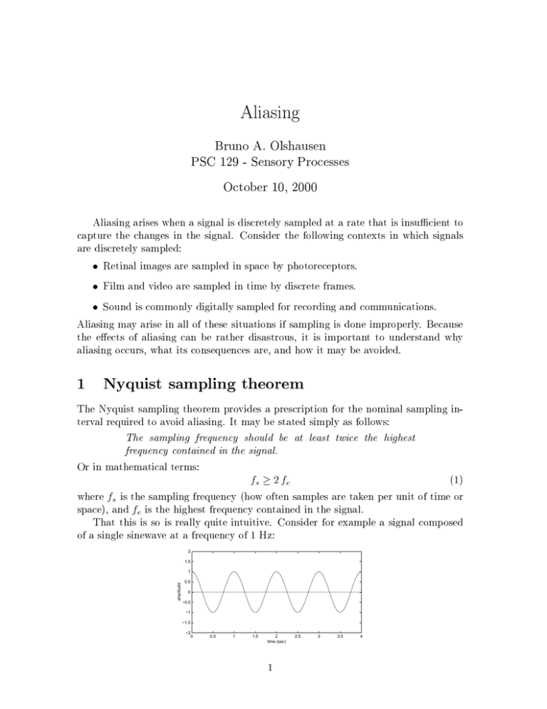
Aliasing
Bruno A. Olshausen
PSC 129 - Sensory Processes
October 10, 2000
Aliasing arises when a signal is discretely sampled at a rate that is insucient to
capture the changes in the signal. Consider the following contexts in which signals
are discretely sampled:
Retinal images are sampled in space by photoreceptors.
Film and video are sampled in time by discrete frames.
Sound is commonly digitally sampled for recording and communications.
Aliasing may arise in all of these situations if sampling is done improperly. Because
the eects of aliasing can be rather disastrous, it is important to understand why
aliasing occurs, what its consequences are, and how it may be avoided.
1 Nyquist sampling theorem
The Nyquist sampling theorem provides a prescription for the nominal sampling interval required to avoid aliasing. It may be stated simply as follows:
The sampling frequency should be at least twice the highest
frequency contained in the signal.
Or in mathematical terms:
fs 2 f c
(1)
where fs is the sampling frequency (how often samples are taken per unit of time or
space), and fc is the highest frequency contained in the signal.
That this is so is really quite intuitive. Consider for example a signal composed
of a single sinewave at a frequency of 1 Hz:
2
1.5
amplitude
1
0.5
0
−0.5
−1
−1.5
−2
0
0.5
1
1.5
2
time (sec)
1
2.5
3
3.5
4
If we sample this waveform at 2 Hz (as dictated by the Nyquist theorem), that is
sucient to capture each peak and trough of the signal:
2
1.5
amplitude
1
0.5
0
−0.5
−1
−1.5
−2
0
0.5
1
1.5
2
time (sec)
2.5
3
3.5
4
If we sample at a frequency higher than this, for example 3 Hz, then there are more
than enough samples to capture the variations in the signal:
2
1.5
amplitude
1
0.5
0
−0.5
−1
−1.5
−2
0
0.5
1
1.5
2
time (sec)
2.5
3
3.5
4
If however we sample at a frequency lower than 2 Hz, for example at 1.5 Hz, then
there are now not enough samples to capture all the peaks and troughs in the signal:
2
1.5
amplitude
1
0.5
0
−0.5
−1
−1.5
−2
0
0.5
1
1.5
2
time (sec)
2.5
3
3.5
4
Note here that we are not only losing information, but we are getting the wrong information about the signal. The person receiving these samples, without any previous
knowledge of the original signal, may well be mislead into thinking that the signal
has quite a dierent form:
2
1.5
amplitude
1
0.5
0
−0.5
−1
−1.5
−2
0
0.5
1
1.5
2
time (sec)
2
2.5
3
3.5
4
From this example, we can see the reason for the term aliasing. That is, the signal
now takes on a dierent \persona," or a false presentation, due to being sampled at
an insuciently high frequency.
Now we are ready to think about the sampling of a complex signal composed of
many frequency components. By Fourier's theorem, we know that any continuous signal may be decomposed in terms of a sum of sines and cosines at dierent frequencies.
For example, the following waveform was composed by adding together sinewaves at
frequencies of 1 Hz, 2 Hz, and 3 Hz:
2
1.5
amplitude
1
0.5
0
−0.5
−1
−1.5
−2
0
0.5
1
1.5
2
time (sec)
2.5
3
3.5
4
According to the Nyquist sampling theorem, the signal must be sampled at twice the
highest frequency contained in the signal. In this case, we have fc=3 Hz, and so the
Nyquist theorem tells us that the sampling frequency, fs, must be at least 6 Hz. And
sure enough, this appears to be sucient:
2
1.5
amplitude
1
0.5
0
−0.5
−1
−1.5
−2
0
0.5
1
1.5
2
time (sec)
2.5
3
3.5
4
Thus, when a signal contains not just one but many dierent frequencies added together, the minimal sampling rate needed to avoid aliasing is just twice whatever the
highest frequency is, irrespective of how many other frequency components there are.
2 Eects of aliasing
2.1 The wagon wheel eect
One common situation in which aliasing occurs is in lm. This is because continuously
varying images are being discretely sampled at a rate of 24 frames/sec. The Nyquist
sampling theorem tells us that aliasing will occur if at any point in the image plane
there are frequency components, or light-dark transitions, that occur faster than fs=2,
which in this case is 12 frames/sec. But in many situations the light-dark transitions
may be occurring faster than this|such as a wagon wheel or propeller rotating at
high speed.
3
Consider a wagon wheel with eight spokes turning at a rate of 3 revolutions per
second (or 180 rpm) in the clockwise direction. In this case, the wagon wheel will
move by one spoke per frame, since
(3 revolutions/sec) (8 spokes/revolution) = 1 spoke/frame
(2)
(24 frames/sec)
Thus, the wagon wheel will appear to stand still! One rarely sees this happen though,
because you have to be awfully lucky for the wheel to be turning at just this speed.
Consider though what would happen if the wagon wheel were turning at a rate
just below this, say at 2.5 revolutions/sec. Now the wheel will move by 83% of the
spoke spacing each frame. So, comparing two adjacent frames of the lm we would
see the following:
Frame 1
Frame 2
The problem the brain faces in viewing these frames in rapid succession is that there
are two interpretations. One interpretation is that the wheel has moved by 83% of
the spoke interval in the clockwise direction. The alternative interpretation is that it
has moved by 17% of the spoke interval in the counter-clockwise direction. It turns
out that the brain prefers the latter interpretation, and so as a result you perceive
the wheel moving backwards (counter-clockwise) at a slower speed than it is actually
moving:
Perceived motion
Actual motion
Frame 1
Frame 2
2.2 Text images
Another place aliasing is often seen is in images of text. This happens for example
when people put an image on their web page that contains some text characters that
has been improperly subsampled. Here is a simple example:
subsampling
4
The image on the right contains half as many samples in each dimension (horizontal
and vertical), and as a result it is now for all practical purposes illegible. In the next
section we will see a simple way to avoid such disastrous eects of aliasing.
3 How to avoid aliasing
The simple way to avoid aliasing of course is to always have enough samples to capture
the spatial or temporal variations in a signal. But there are many situations in which
the sample rate may be limited|for example, lm is limited to 24 frames/sec, or you
may be designing a web page where the images need to be a minimum number of pixels
so they download quickly. So, if the sampling rate fs is xed, then there is only one
other parameter we can play with, and that is the highest frequency contained in the
signal, fc. This can be done by lowpass ltering, or in layman's terms, \smoothing."
The easiest way to smooth a signal is to blur it. In lm this is easily done by
adjusting the lens so the image is a bit out of focus. The more out of focus it is,
the lower the spatial-frequency content of the image becomes. And as the spatialfrequency content is lowered, the temporal frequency content is also lowered. Blurring
is often used by lm directors to eliminate aliasing from a scene. For example, when
lming a shot where a car is racing by, it would be a mistake to keep the car in focus.
The image of the car is usually purposefully de-focussed so as to eliminate the jerky
appearance of motion, which breaks the illusion of reality in lm. Oftentimes though,
directors will not bother to eliminate aliasing in the form of backwards moving wheels,
or they may even prefer to keep it for \visual eect."
Blurring may be easily accomplished on digital images by ltering (or convolving)
with a mask that averages together the values of several neighboring pixels. Such an
operation is usually provided in image manipulation programs such as Photoshop.
3.1 Text images revisited
Now that we know how to avoid aliasing, we can form a properly subsampled version
of our text image by blurring the image a bit before subsampling:
smoothing
subsampling
Note that the subsampled text image is now at least legible, yet it has the same
number of pixels as the image in the previous example. This technique is also known
5
as \anti-aliasing" in the computer graphics community.
3.2 Natural images
The avoidance of aliasing is also important in the design of the eye. For example, in
the human eye the lens lters out any spatial variations ner than 60 cycles/degree.
The Nyquist theorem tells us in this case that the photoreceptor spacing should be
at least 120 sample/degree, which is exactly what we have! Consider though what
the sampled retinal image might look like if this were not the case:
blur
sample
sample
At upper left is shown a natural image that may typically fall on the retina, and
below this is shown the result of subsampling the image without properly blurring
beforehand. Compare this to the sampled version after blurring (lower right). It is
not dicult to see why nature has gone to the eort it has to match photoreceptor
spacing with the point-spread function (spatial-frequency cuto) of the lens.
6