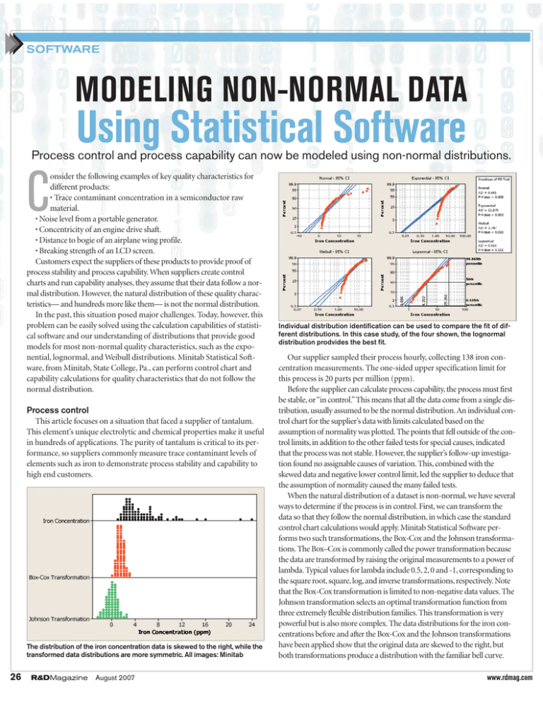
SOFTWARE
MODELING NON-NORMAL DATA
Using Statistical Software
Process control and process capability can now be modeled using non-normal distributions.
C
onsider the following examples of key quality characteristics for
different products:
• Trace contaminant concentration in a semiconductor raw
material.
• Noise level from a portable generator.
• Concentricity of an engine drive shaft.
• Distance to bogie of an airplane wing profile.
• Breaking strength of an LCD screen.
Customers expect the suppliers of these products to provide proof of
process stability and process capability. When suppliers create control
charts and run capability analyses, they assume that their data follow a normal distribution. However, the natural distribution of these quality characteristics— and hundreds more like them— is not the normal distribution.
In the past, this situation posed major challenges. Today, however, this
problem can be easily solved using the calculation capabilities of statistical software and our understanding of distributions that provide good
models for most non-normal quality characteristics, such as the exponential, lognormal, and Weibull distributions. Minitab Statistical Software, from Minitab, State College, Pa., can perform control chart and
capability calculations for quality characteristics that do not follow the
normal distribution.
Process control
This article focuses on a situation that faced a supplier of tantalum.
This element’s unique electrolytic and chemical properties make it useful
in hundreds of applications. The purity of tantalum is critical to its performance, so suppliers commonly measure trace contaminant levels of
elements such as iron to demonstrate process stability and capability to
high end customers.
The distribution of the iron concentration data is skewed to the right, while the
transformed data distributions are more symmetric. All images: Minitab
26
R&DMagazine
August 2007
Individual distribution identification can be used to compare the fit of different distributions. In this case study, of the four shown, the lognormal
distribution prodvides the best fit.
Our supplier sampled their process hourly, collecting 138 iron concentration measurements. The one-sided upper specification limit for
this process is 20 parts per million (ppm).
Before the supplier can calculate process capability, the process must first
be stable, or “in control.” This means that all the data come from a single distribution, usually assumed to be the normal distribution. An individual control chart for the supplier’s data with limits calculated based on the
assumption of normality was plotted. The points that fell outside of the control limits, in addition to the other failed tests for special causes, indicated
that the process was not stable. However, the supplier’s follow-up investigation found no assignable causes of variation. This, combined with the
skewed data and negative lower control limit, led the supplier to deduce that
the assumption of normality caused the many failed tests.
When the natural distribution of a dataset is non-normal, we have several
ways to determine if the process is in control. First, we can transform the
data so that they follow the normal distribution, in which case the standard
control chart calculations would apply. Minitab Statistical Software performs two such transformations, the Box-Cox and the Johnson transformations. The Box–Cox is commonly called the power transformation because
the data are transformed by raising the original measurements to a power of
lambda. Typical values for lambda include 0.5, 2, 0 and -1, corresponding to
the square root, square, log, and inverse transformations, respectively. Note
that the Box-Cox transformation is limited to non-negative data values. The
Johnson transformation selects an optimal transformation function from
three extremely flexible distribution families. This transformation is very
powerful but is also more complex. The data distributions for the iron concentrations before and after the Box-Cox and the Johnson transformations
have been applied show that the original data are skewed to the right, but
both transformations produce a distribution with the familiar bell curve.
www.rdmag.com
Finding an appropriate distribution
Transformations clearly can provide a solution to the non-normality
issue. However, suppliers may not appreciate the resulting loss of physical
connection with the measurement. In our example, if the optimal lambda
is zero, then the analysis is performed on the log of the iron concentration
measurements, rather than the original measurements. Conceptualizing
what the log of the measurements means can be challenging.
A second approach is to find a non-normal distribution that fits the
data. Many non-normal distributions can be used to model a response,
but if an alternative to the normal distribution is going to be viable, the
exponential, lognormal, and Weibull distributions usually work. The
extreme value and gamma distributions have their applications, but if
neither the normal, exponential, lognormal, nor Weibull distributions
provide a good fit, the data may be a mixture of a number of different
populations. In that case, the supplier needs to separate the data by population and analyze each individually.
The supplier can assess the fit for each distribution based on how well
the plotted points follow the middle blue model line. In this case, the exponential distribution is a very poor model for the iron concentration data,
while the lognormal distribution appears to provide a good model. Additional support for the lognormal model can be seen in the high p-value (pvalue = 0.111) for the Anderson-Darling goodness-of-fit test. This p-value
indicates that there is not enough evidence in the data to reject the null
hypothesis that the lognormal distribution is a good fit for the iron data.
Based on the results of this distribution identification analysis, we can conclude that the lognormal distribution is a good model for the iron data.
Now that we know the lognormal distribution provides a good model
for the data, we can use that distribution to construct the proper individuals chart. A standard individuals chart with +/- 3 ␴ control limits for
normally distributed data has a false alarm probability of ␣=0.0027 with
control limits at the 0.135th and 99.865th percentiles of the distribution
and a center line at the at the 50th percentile. To construct an equivalent
control chart, Minitab determines the same percentiles for the lognormal
distribution that describes the iron data. These percentiles are shown on
the lognormal probability plot. The control chart based on these percentiles indicates that the process is in control, where only common cause
variation is seen in the iron concentration values. This was not the conclusion initially reached when the distribution was improperly assumed
to be normal. By evaluating the distribution of the data, we have revealed
that the process is stable, with the distribution of the data well described
by the lognormal family of distribution curves.
Process capability
Determining process capability quantitatively answers the question “Is
my process capable of meeting my customer’s specifications?” The answer
can take many forms. The most common capability estimate is Cpk, which
for normally distributed data takes the familiar form of the distance from
the data average to the closest specification, divided by 3 standard deviations. A more general calculation of Cpk, is derived as follows:
Cp = Allowable Spread = UpperSpec – Lower Spec
Process Spread
X0.99865 – X0.00135
where X0.99865 and X0.00135 are the 0.135th and 99.865th percentiles of the
distribution that describes the quality characteristic of interest. If Cpl
and Cpu are the acceptable spread with respect to the upper and lower
www.rdmag.com
The lognormal distribution is one of 13 non-normal distributions offered in
Minitab’s non-normal capability analysis.
specifications defined as follows:
Cpl = Median – LowerSpec
Median – X0.00135
Cpu = UpperSpec — Median
X0.99865 — Median
then Cpk equals the minimum of Cpl and Cpu. Cpk is an indicator of
the percentage of the parts beyond the upper or lower specification,
whichever percentage is greater. When the data are not normally distributed, Minitab can estimate the distribution percentiles and compute the
capability estimate. For our iron concentration measurements, Cpk is
calculated as follows:
[
20 — 4.203
]
Cpk = min[Cpl,Cpu] = min *, 25.302 — 4.203 = 0.75
Minitab’s non-normal capability analysis was carried out using an
upper specification of 20 ppm. (No lower spec was available, so Cpl
does not apply in this case.) Similar to the probability output, the histogram of the capability output shows that the data are modeled well
using a lognormal distribution. The process capability is equal to 0.75
with an expected overall performance of approximately 4,567 ppm
falling outside of the specification limit. (Note that Minitab uses Ppk
rather than Cpk when reporting the actual process capability for nonnormal data, though the calculations are the same as those referenced
above. Minitab refers to Cpk only when reporting the potential capability of a process.)
Getting away from normal
Researchers are frequently asked to evaluate process stability and capability for key quality characteristics that follow non-normal distributions. In the past, demonstrating process stability and capability
required the assumption of normally distributed data. However, if data
do not follow the normal distribution, the results generated under this
assumption will be incorrect. Whether you decide to transform data to
follow the normal distribution or identify an appropriate non-normal
distribution model like this tantalum supplier did, Minitab Statistical
Software can be used to accurately verify process stability and calculate
process capability for non-normal quality characteristics.
—Lou Johnson,
Technical Trainer, Minitab, Inc.
RESOURCES
쑲 Minitab, Inc., State College, Pa., 814-238-3280, www.minitab.com
August 2007
R&DMagazine
27