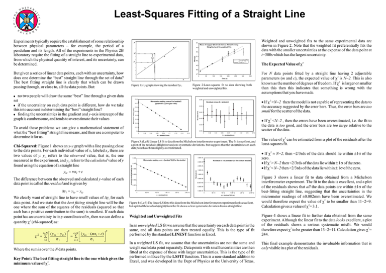
Least-Squares Fitting of a Straight Line
Experiments typically require the establishment of some relationship
between physical parameters – for example, the period of a
pendulum and its length. All of the experiments in the Physics 2B
laboratory require the fitting of a straight line to experimental data,
from which the physical quantity of interest, and its uncertainty, can
be determined.
y
Weighted and unweighted fits to the same experimental data are
shown in Figure 2. Note that the weighted fit preferentially fits the
data with the smaller uncertainties at the expense of the data point at
t=300s which has the largest uncertainty.
54
Mass of Copper Electrode Versus Time Showing
Weighted and Unweighted Fits
53
52
Mass (g)
yio
Dyi
yic
51
Unweighted Fit
50
The Expected Value of c2
Weighted Fit
49
48
For N data points fitted by a straight line having 2 adjustable
2
parameters (m and c), the expected value of c is N-2. This is also
2
known as the number of degrees of freedom. If c is larger or smaller
than this then this indicates that something is wrong with the
assumptions that you have made.
47
0
xi
100
150
200
250
300
350
Time (s)
Figure 1: x-y graph showing the residual Dyi.
! no two people will draw the same “best” line through a given data
set
! if the uncertainty on each data point is different, how do we take
this into account in determining the “best” straight line?
! finding the uncertainties in the gradient and y-axis intercept of the
graph is cumbersome, and tends to overestimate their values
50
x
Figure 2:Least-squares fit to data showing both
weighted and unweighted fits.
15.8
0.005
Micrometer reading versus N x lambda/2
(gradient is (–) the gear ratio)
15.7
· If c2 >N-2 then the model is not capable of representing the data to
the accuracy suggested by the error bars. Thus, the error bars are too
small for the scatter of the data.
Residual versus N x lambda/2
Micrometer reading (mm)
0.003
15.6
15.5
Residual (mm)
But given a series of linear data points, each with an uncertainty, how
does one determine the “best” straight line through the set of data?
The best fitting straight line is clearly that which can be drawn
passing through, or close to, all the data points. But:
15.4
15.3
0.001
-0.001
· If c2 <N-2 , then the errors have been overestimated, i.e. the fit to
the data is too good, and the error bars are too large relative to the
scatter of the data.
15.2
-0.003
To avoid these problems we can give a mathematical statement of
what the “best fitting” straight line means, and then use a computer to
determine it for us.
The difference between the observed and calculated y-value of each
data point is called the residual and is given by
0
0.02
0.04
0.06
0.08
0.1
0.12
0.14
0
0.16
0.02
0.04
0.06
0.08
0.1
0.12
0.14
0.16
N x lambda/2 (mm)
N x lambda/2 (mm)
3.00E-05
0.006
Micrometer reading vs n x (lambda^2)/2 for Na doublet
Residual vs n x (lambda^2)/2 for sodium doublet
2.50E-05
0.005
2.00E-05
0.004
0.003
1.50E-05
5.00E-06
0.00E+00
0.001
0
We clearly want of straight line to have small values of Dyi for each
data point. And we state that the best fitting straight line will be the
one where the sum of the squares of the residuals (squared so that
each has a positive contribution to the sum) is smallest. If each data
point has an uncertainty in its y-coordinate of si, then we can define a
quantity c2 (chi-squared) as:
2
i = N é ( y - ( mx + c ) ù
i= N é ( y - y ) ù
io
i
ic
c 2 = å ê io
ú = å ê
ú
si
si
i =1 ë
i =1 ë
û
û
-1.00E-05
0
2
Where the sum is over the N data points.
Key Point: The best fitting straight line is the one which gives the
minimum value of c2.
5E-13
1E-12
1.5E-12
2E-12
n x lambda/2 (m)
2.5E-12
· If c2 » N-2, then ~2/3rds of the data should lie within ±1s of the
zero.
· If c2 > N-2 then <2/3rds of the data lie within ± 1s of the zero.
· If c2 < N-2 then >2/3rds of the data lie within ± 1s of the zero.
1.00E-05
0.002
-5.00E-06
Dyi = yio - yic
The value of c can be estimated from a plot of the residuals after the
least-squares fit.
2
Figure 3: (Left) Linear LS fit to data from the Michelson interferometer experiment. The fit is excellent, and
a plot of the residuals (Right) reveals no systematic deviations, but suggests that the uncertainties on each
data point have been slightly overestimated.
Residual (m)
yic = mxi + c
-0.005
15
micromter reading/gearing (m)
Chi-Squared: Figure 1 shows an x-y graph with a line passing close
to the data points. For each individual value of x, labeled xi, there are
two values of y: yio refers to the observed value, that is, the one
measured in the experiment, and yic refers to the calculated value of y
found using the equation of a straight line
15.1
0
5E-13
1E-12
1.5E-12
2E-12
2.5E-12
n x (lambda^2)/2 (m)
Figure 4: (Left) The linear LS fit to this data from the Michelson interferometer experiment looks excellent,
but a plot of the residuals (right) from the fit shows a clear systematic deviation from a straight line.
Weighted and Unweighted Fits
In an unweighted LS fit we assume that the uncertainty on each data point is the
same, and all data points are then treated equally. This is the type of fit
performed by the standard LINEST function in Excel.
In a weighted LS fit, we assume that the uncertainties are not the same and
weight each data point separately. Data points with small uncertainties are then
fitted at the expense of those with larger uncertainties. This is the type of fit
performed in Excel by the LSFIT function. This is a non-standard addition to
Excel, and was developed in the Dept of Physics at the University of Texas,
Figure 3 shows a linear fit to data obtained from a Michelson
interferometer experiment. The fit to the data is excellent, and a plot
of the residuals shows that all the data points are within ±1s of the
best-fitting straight line, suggesting that the uncertainties in the
micrometer readings of ±0.002mm have been overestimated. We
2
would therefore expect the value of c to be smaller than 11-2=9.
2
Calculation gives a value of c = 3.1.
Figure 4 shows a linear fit to further data obtained from the same
experiment. Although the linear fit to the data looks excellent, a plot
of the residuals shows a serious systematic misfit. We would
therefore expect c2 to be greater than 13-2=11. Calculation gives c2=
244.
This final example demonstrates the invaluable information that is
only visible in a plot of the residuals.