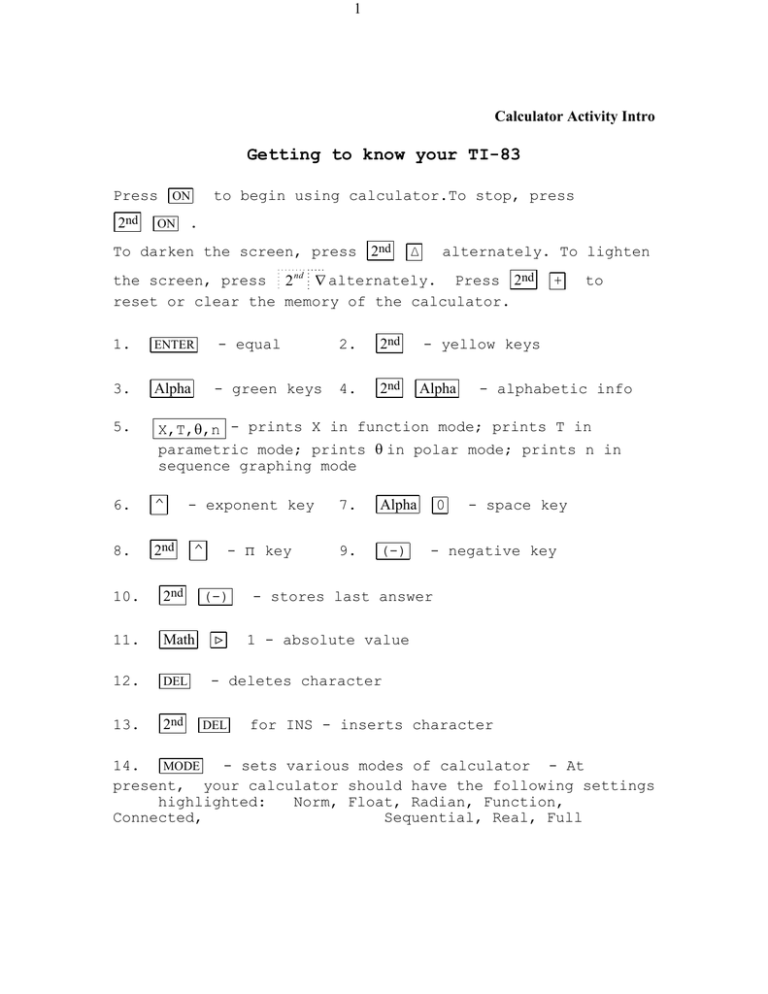
1
Calculator Activity Intro
Getting to know your TI-83
Press ON
2nd
ON
to begin using calculator.To stop, press
.
To darken the screen, press 2nd
∆
alternately. To lighten
the screen, press 2 nd  alternately. Press 2nd
reset or clear the memory of the calculator.
- equal
2.
2nd
- yellow keys
- green keys
4.
2nd
Alpha
+
to
1.
ENTER
3.
Alpha
5.
X,T,,n - prints X in function mode; prints T in
parametric mode; prints in polar mode; prints n in
sequence graphing mode
6.
^
8.
2nd
- exponent key
^
10.
2nd
11.
Math
12.
DEL
13.
2nd
- π key
(-)

7.
Alpha
9.
(-)
0
- alphabetic info
- space key
- negative key
- stores last answer
1 - absolute value
- deletes character
DEL
for INS - inserts character
14.
MODE
- sets various modes of calculator - At
present, your calculator should have the following settings
highlighted:
Norm, Float, Radian, Function,
Connected,
Sequential, Real, Full
2
15.
MATH
16.
2nd
-
1.
2.
3.
4.
5.
6.
7.
8.
9.
10.
display answer as a fraction
display answer as a decimal
cube a number
take the cube root of a number
take the xth root of a number
minimum of a function
maximum of a function
numerical derivative
function integral
solves for any variable in an equation
- (for TEST) -
MATH
1.
2.
3.
4.
5.
6.
17.
2nd
MATRIX
=
≠
>
≥
<
≤
- (for ANGLE) - 1. degree notation
2. minute notation
3. radian notation
4. displays as
degree/minute/second
5. - 8. used to change from
rectangular coordinates to polar coordinates or from polar
to rectangular
18.
PRGM
19.
2nd
PRGM
EXEC EDIT NEW
- (for DRAW) -
1.
Clr draw
2. Line
3. Horizontal
4. Vertical
5. Tangent
6. Draw function
7. Shade
8. Draw inverse
9. Draw circle
10. adds text to graph
A. free-form drawing tool
3
Graphing keys - top row of calculator
1. Y= - allows you to enter up to ten separate equations
2. WINDOW - sets dimensions of viewing rectangle
3. ZOOM - allows you to adjust the viewing rectangle
4. TRACE - allows you to find a specific point on a graph
5. GRAPH - draws the graph of a function
Using the viewing rectangle
The viewing rectangle on the TI-83 is 94 pixels (A pixel is a picture element.) by
62 pixels. It is useful when graphing to have a "friendly window" in order to
avoid distortion in the graph and to avoid obtaining non-integer values when
using the trace function of the TI-83. In fact, a program helps alleviate these
problems.
A Friendly Window
Program:WINDOW
:ClrHome
:Disp "SCALE FACTOR ="
:Input F
:-4.7FXmin
:4.7FXmax
:FXscl
:-3.1FYmin
:3.1FYmax
:FYscl
:Stop
Save Graphing Window
Program:SAVWINDO
:XminA
:XmaxB
:XsclC
:YminD
:YmaxE
:YsclF
:Stop
4
Recall Graphing Window
Program:RECWINDO
:AXmin
:BXmax
:CXscl
:DYmin
:EYmax
:FYscl
:Stop
Basic Calculator Operations
37  4  3 3
16  1  2 2
1.
Simplify:
2.
Simplify:
3.
Let a = 2 and b = 4. Evaluate the expression: 3ab - 1
3 2 4 2
Screen displays:
4.
ENTER
When you were collecting the data required for a water temperature
project, you forgot to take temperature readings in degrees Celsius. The
following formula is used to convert from degrees Fahrenheit to
degrees Celsius:
5
5(F  32)
C  ( F  3 2 ) or
C
9
9
a. Change 50°F to degrees Celsius.
b. Change 103°F to degrees Celsius.
5.
Approximate the value of each expression to the nearest thousandth:
a. 3 15
b. 5 46
5
6.
Evaluate the function, f(x) = 2x2 – 3x + 7 for x = 2, x = –1, x = 0, and
x = 141.3456.
Store f(x) = 2x2 – 3x + 7 in Y= .
Press Y= and type the function in Y1.
(You can choose any Y you wish.)
Press 2nd [QUIT]. Press
VARS  ENTER ENTER .
Press
(
2
)
.
Press ENTER .
Follow the same procedure in order to
evaluate f(x) for each value of x.
6
Calculator Activity 1
PLOTTING POINTS FROM DATA
Entering Data into Columns
The data in the chart below is water temperature measured at the same site over
a period of weeks. L1 contains the number of the week and L2 contains the
temperature in degrees Celsius recorded for the week. These lists must have the
same number of data points.
L1
L2
1
46
2
41
3
51
4
39
5
38
7
41
10
42
12
47
13
37
15
39
16
41
Press
Error!.
Press 1 (to select Edit) .
Enter the X values in L1. Press ENTER
after each entry to go to the next line.
When finished with the X values, press  to place the cursor at the beginning
of L2. Enter all Y values in L2. (The screen below does not display the entire data
set.)
7
Press 2nd [QUIT].
8
Plotting Data Points
To graph the data points in the lists, L1 and L2:
Press 2nd
[STAT PLOT].
Press ENTER .
Press ENTER . (The cursor is
blinking on the On. By pressing enter,
you are turning on stat plot 1. )
Use the down arrow to move to the
Type line. If necessary, use the left
arrow to move to the scatter plot icon.
Use the down arrow to move to Xlist.
Press 2nd 1.
Use the down arrow to move to Ylist.
Press 2nd 2.
9
Press 2nd [QUIT]. Press
WINDOW
and choose appropriate settings for the
data.
Press GRAPH . The scatter plot at
the right is only one way to represent
the data graphically.
Press 2nd [STAT PLOT]. Choose
line graph. Press 2nd [QUIT].
Press GRAPH . A line graph is
another way to represent data
graphically.
Press 2nd [STAT PLOT]. Choose a
bar graph or histogram. L1 is in Xlist.
Press 2nd 2 to put L2 in Freq. Press
2nd [QUIT].
Press GRAPH . Note: WINDOW
settings are 0,18,1,0,55,5,1.
Temperature by week
Before you go to another activity, turn "Off" all stat plots.
10
Calculator Activity 2
GRAPHING WITH TI-83
Graphing an Equation with TI-83
1. Solve the equation for y.
2. Enter the equation in Y= .
3. Determine an appropriate viewing rectangle. Enter the values in WINDOW .
4. Press GRAPH .
Example 1: Graph 2x + 3y = 9. An appropriate WINDOW is –9, 9, 1, –6, 6, 1, 1.
Answer: Solve 2x + 3y = 9 for y.
2
Store y = – 3 x + 3 in Y1.
Press GRAPH .
Example 2: Graph y = 2x2 – 5.
Answer: Store y = 2x2 – 5 in Y1.
Press GRAPH .
Example 3: Graph y =
Answer: Store y =
2x + 6 .
2x + 6 in Y1.
Press GRAPH .
11
2
Example 4: Graph y = x–3 . Since this equation represents a rational function, we know
that we have to eliminate any value that makes the denominator equal to 0. This
function has a vertical asymptote at x = 3.
2
Answer: Store y = x–3 in Y1.
Press GRAPH .
Notice that the graph should consist of two unconnected portions - one to the left of x =
3 and the other to the right of x = 3. To eliminate the problem with the graph, change
the mode of the calculator from connected to dot. There are two ways in which to make
this change.
Press Y= . Arrow to the
left as far as possible.
Press ENTER repeatedly
to rotate through the
graph styles. Stop on
Press GRAPH .
This graph is more
difficult to read because
it uses a collection of dots
rather than a smooth curve.
If you choose window settings in which the vertical asymptote is the center of the xvalues, you will be able to use connected mode and to obtain an accurate graph. In this
example, x = 3 is the vertical asymptote. Change the window settings so that
x = 3 is exactly the middle value between Xmin and Xmax.
Using the trace cursor
shows that the function is
undefined when x = 3.
12
Example 5: Graph y = x  2 .
Answer: Store y = x  2 in Y1.
Press GRAPH .
Example 6: Graph y = x 3  1
Answer: Store y = x 3  1 in Y1.
Press GRAPH .
1
Example 7: Graph y = – x+3 .
1
Answer: Store y = – x+3 in Y1.
Press GRAPH .
In all of the previous examples, the WINDOW settings remained the same. The ratio
of x to y should be 3 to 2 in order to obtain a graph with little distortion. You will have
to choose an appropriate WINDOW .
Example 8: Graph y = – x 3  2x 2  3x  7
Answer: Store y = – x 3  2x 2  3x  7
in Y1.
Press GRAPH .
Is this the correct
graph?
13
Choose a more appropriate WINDOW .
You may have to experiment to
determine the most appropriate
window settings. You could run
program: WINDOW and change the
scale factor until you have a correct
graph.
The TI-83 has a table of values that may be used to list specific values for the
independent variable, x, and the computed values of the dependent variable, y.
For example, complete a table of values for the function y = –3x + 5 where x begins at –
10 and is incremented by 1 unit.
Press 2nd [TBLSET].
This screen indicates that
the table will start at 0 and
have an increment of 1.
Both variables will appear
automatically.
Change table start to –10
and leave ∆Tbl = 1.
Use the arrow keys to
Enter y = –3x + 5 in Y= . scroll down the x- and yvalues. You can also
Press 2nd [GRAPH].
scroll up the x list and
the y list.
Intercepts
The table of values may be used to find the x-intercept(s) and y-intercept of a curve.
Alternately, CALC 1 (for value) may be used to find the value of the y-intercept and
CALC 2 (for zero) may be used to find the value of the x-intercepts, if they exist.
Store y = x2 – 6x + 8
in Y1.
Choose an appropriate
WINDOW .
14
Press GRAPH .
Press 2nd [CALC] 1.
The point (0,8) is the y-intercept.
To find the x-intercepts, press
2nd [CALC] 2. Select a left
bound by pressing ENTER to
Enter 0 for X.
Use right arrow to move
the cursor to the right of
the x-intercept. Press
Place the cursor on the
x-intercept and press
ENTER .
ENTER .
the left of an x-intercept.
One of the x-intercepts is (2,0). Follow the above procedure to determine the other xintercept which is (4,0).
15
Calculator Activity 3
PIECEWISE-DEFINED FUNCTIONS
Graphing piecewise-defined functions
A function defined by two or more equations over a specified domain is called a
if x  2
2x – 3
piecewise-defined function. Graph f(x)  
2
0.2x + 2 if x > 2
The screen shows a way to enter f(x)
into the calculator.
The screen shows another way to enter
f(x) into the calculator.
Evaluating a Function
To evaluate a piecewise-defined function for a specific value of x, enter the
following into the calculator.
Press VARS ~ ENTER ENTER
Press
(
The table can also be used to evaluate a function.
2
)
ENTER
16
Calculator Activity 4
Linear Regression with TI-83
The winning times (in minutes) in the women's 400-meter freestyle swimming
event in the Olympics from 1948 to 1992 are given by the following ordered
pairs.
(1948, 5.30)
(1972, 4.32)
(1952, 5.20)
(1976, 4.16)
(1956, 4.91)
(1980, 4.15)
(1960, 4.84)
(1984, 4.12)
(1964, 4.72)
(1988, 4.06)
(1968, 4.53)
(1992, 4.12)
Enter the data in your calculator. If necessary, clear L1 and L2. (Highlight L1 ,
press CLEAR and ENTER . Repeat for L2. ) Let t = 0 represent 1940.
Press 2nd [QUIT].
Press GRAPH .
Choose an appropriate
window for the data.
All of the data will not
show on the screen.
Press 2nd [QUIT].
Press STAT
Press ENTER .
~ 4 (for
LinReg(ax+b)). Press
2nd [L1] ¢ 2nd [L2]
¢ VARS ~
ENTER
ENTER .
Press Y= .
Press GRAPH .