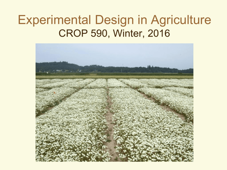
Experimental Design in Agriculture
CROP 590, Winter, 2016
Why conduct experiments?...
 To explore new technologies, new crops, and
new areas of production
 To develop a basic understanding of the factors
that control production
 To develop new technologies that are superior
to existing technologies
 To study the effect of changes in the factors of
production and to identify optimal levels
 To demonstrate new knowledge to growers and
get feedback from end-users about the
acceptability of new technologies
What is a designed experiment?
 Treatments are imposed (manipulated) by
investigator using standard protocols
 May infer that the response was due to the
treatments
Potential pitfalls
 As we artificially manipulate nature, results may not
generalize to real life situations
 As we increase the spatial and temporal scale of
experiments (to make them more realistic), it becomes
more difficult to adhere to principles of good
experimental design
What is an observational study?
 Treatments are defined on the basis of existing
groups or circumstances
 Uses
– Early stages of study – developing hypotheses
– Scale of study is too large to artificially apply treatments
(e.g. ecosystems)
– Application of treatments of interest is not ethical
 May determine associations between treatments and
responses, but cannot assume that there is a cause
and effect relationship between them
 Testing predictions in new settings may further
support our model, but inference will never be as
strong as for a designed (manipulative) experiment
Some Types of Field Experiments
(Oriented toward Applied Research)
 Agronomy Trials
–
–
–
–
Fertilizer studies
Time, rate and density of planting
Tillage studies
Factors are often interactive so it is good to include
combinations of multiple levels of two or more factors
– Plot size is larger due to machinery and border effects
 Integrated Pest Management
– Weeds, diseases, insects, nematodes, slugs
– Complex interactions betweens pests and host plants
– Mobility and short generation time of pests often create
challenges in measuring treatment response
Types of Field Experiments (Continued)
 Plant Breeding Trials
– Often include a large number of treatments (genotypes)
– Initial assessments may be subjective or qualitative using
small plots
– Replicated yield trials with check varieties including a long
term check to measure progress
 Pasture Experiments
– Initially you can use clipping to simulate grazing
– Ultimately, response measured by grazing animals so plots
must be large
– The pasture, not the animal, is the experimental unit
Types of Field Experiments (Continued)
 Experiments with Perennial Crops
– Same crop on same plot for two or more years
– Effects of treatments may accumulate
– Treatments cannot be randomly assigned each year so it is not
possible to use years as a replication
– Large plots will permit the introduction of new treatments
 Intercropping Experiments
– Two or more crops are grown together for a significant part of the
growing season to increase total yield and/or yield stability
– Treatments must include crops by themselves as well as several
intercrop combinations
– Several ratios and planting configurations are used so number of
treatments may be large
– Must be conducted for several years to assess stability of system
Types of Field Experiments
(Continued)
 Rotation Experiments
– Determine effects of cropping sequence on target crop, pest or
pathogen, or environmental quality
– Treatments are applied over multiple cropping seasons or years,
but impact is determined in the final season
 Farming Systems Research
–
–
–
–
–
–
To move new agricultural technologies to the farm
A number of farms in the target area are identified
Often two large plots are laid out - old versus new
Should be located close enough for side by side comparisons
May include “best bet” combinations of several new technologies
Recent emphasis on farmer participation in both development
and assessment of new technologies
The Scientific Method
 Formulation of an
H ypothesis
 P lanning an experiment to objectively test the
hypothesis
 Careful observation and collection of
D ata from
the experiment
 I nterpretation of the experimental results
Steps in Experimentation
H
Definition of the problem
Statement of objectives
P
Selection of treatments
Selection of experimental material
Selection of experimental design
Selection of the unit for observation and the number of replications
Control of the effects of the adjacent units on each other
Consideration of data to be collected
Outlining statistical analysis and summarization of results
D
Conducting the experiment
I
Analyzing data and interpreting results
Preparation of a complete, readable, and correct report
The Well-Planned Experiment
 Simplicity
– don’t attempt to do too much
– write out the objectives, listed in order of priority
 Degree of precision
– appropriate design
– sufficient replication
 Absence of systematic error
 Range of validity of conclusions
– well-defined reference population
– repeat the experiment in time and space
– a factorial set of treatments also increases the range
 Calculation of degree of uncertainty
Hypothesis Testing
 H0:  = ɵ HA:   ɵ or H0: 1= 2 HA: 1 2
/2
/2

critical value
 If the observed (i.e., calculated) test statistic is greater
than the critical value, reject H0
 If the observed test statistic is less than the critical value,
fail to reject H0
Hypothesis Testing
 The concept of a rejection region (e.g.  = 0.05)
is not favored by some statisticians
 It may be more informative to:
– Report the p-value for the observed test statistic
– Report confidence intervals for treatment means
Hypothesis testing
 It is necessary to define a rejection region to determine
the power of a test
Decision
Accept H0
Reject H0
Reality

H0 is true
1 = 2
Correct
HA is true
1  2

1-
Type II error
Power
Type I error
Power of the test
H0
HA
1–
p
/2
1–

/2
 Power is greater when
– differences among treaments are large
– alpha is large
– standard errors are small
Review - Corrected Sum of Squares
 Definition formula
n

SS Y   Yi  Y
i1

2
 Computational formula
– common in older textbooks
uncorrected
sum of squares
correction
factor


  Yi 
n
i1


2
SS Y   Yi 
n
i1
n
2
t tests – one sample
To test the hypothesis that the mean of a single
population is equal to some value:
Y  0
t
sY
Compare to critical t
for n-1 df for a given 
(0.05 in this graph)
standard error of the mean
s2
where s Y 
n
df = 
df = n-1
df = 6
df = 3
t tests – two samples, equal variance
To compare the mean of two populations with
equal variances and equal sample sizes:
Y1  Y 2
t
s Y1  Y2
standard error of the difference
where
s Y1 Y2 
2
P
2s
n
df = 2(n-1)
The pooled s2 (sP2 ) should be the average of
the variance estimates of the two samples
t tests – unequal sample size
To compare the mean of two populations with
equal variances and unequal sample sizes:
Y1  Y 2
t
sY1  Y2
where s Y1 Y2
1 1
 s    df = (n1-1) + (n2-1)
 n1 n2 
2
P
The pooled s2 (sP2 ) should be a weighted average of the
variance estimates from the two samples
2
2
𝑛
−
1
𝑠
+
𝑛
−
1
𝑠
𝑆𝑆1 + 𝑆𝑆2
1
2
1
2
𝟐
𝒔𝑷 =
=
𝑛1 − 1 + 𝑛2 − 1
𝑛1 − 1 + 𝑛2 − 1
Paired t test
 When observations are paired, it may be beneficial
to use a paired t test
– for example, feeding rations given to animals from the
same litter
 t2 = F in a Completely Randomized Design (CRD)
when there are only two treatment levels
 Paired t2 = F in a RBD (Randomized Complete
Block Design) with two treatment levels
Measures of variation
 Sample variance
 Standard deviation
SSY
s 
n1
2
s
 Coefficient of Variation
2
s
CV% 
x 100
Y
– Expresses the standard deviation as a proportion of the
mean
– Varies from 0 to 100 (not on original scale)
– Used to compare precision of data from similar types of
experiments
Confidence Intervals
 100(1-)% confidence interval for a mean (𝐿𝑌 )
Y  t  ,df
2
s
n
If we repeatedly obtained samples of the same
size from a population, and constructed
confidence intervals, we would expect 95% of
those intervals to contain the true mean.
 100(1-)% confidence interval for a difference
between two means (𝐿𝑌1−𝑌2 )
Y  Y   t
1
2
 ,df
2s2
n
Measures of Variation
s (standard deviation)
Y
s2
n
CV (coefficient of variation)
s2
* 100
Y
t ,df
se (standard error of a mean)
L (Confidence Interval for a mean)
2
s
n
sY1Y2
t ,df 2
2
(standard error
of a difference
between means)
2s2
n
Y  t  ,df
t ,df
s2
n
2
LSD (Least Significant Difference between means)
L(Confidence Interval for a difference between means)
t ,df
2s2
n
Y  Y   t
1
2
 ,df
2s2
n