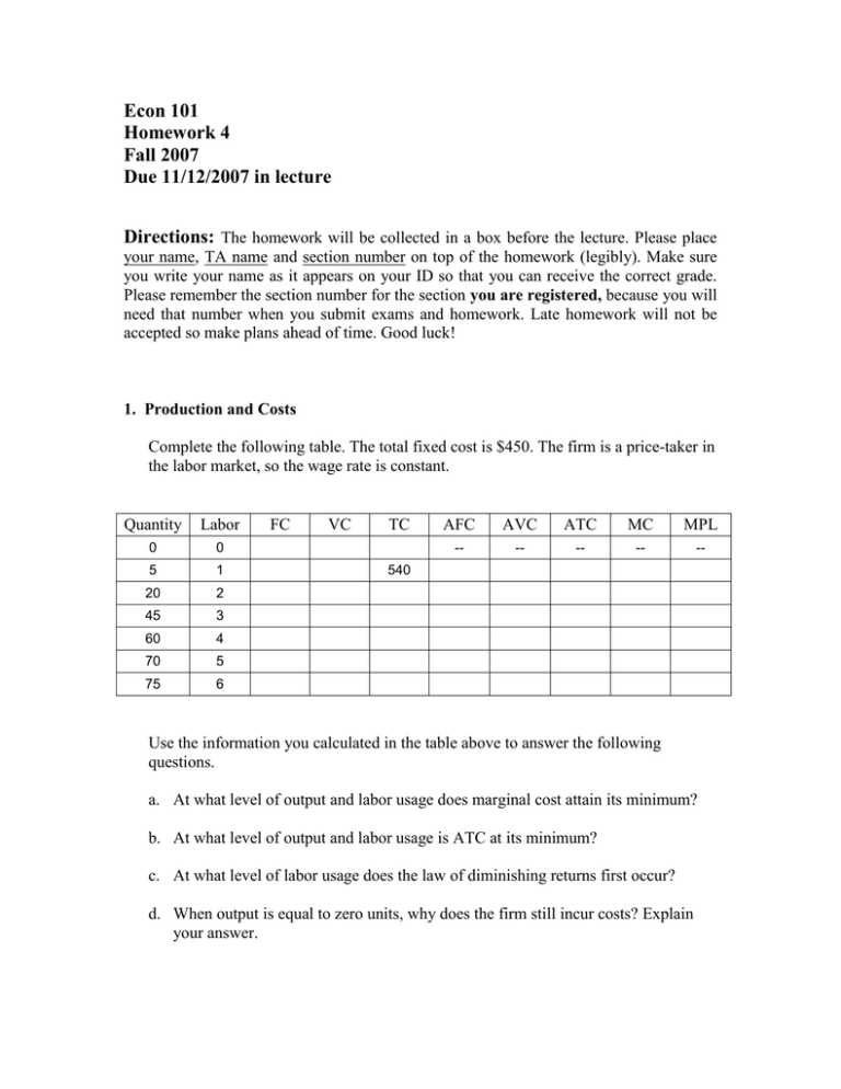
Econ 101
Homework 4
Fall 2007
Due 11/12/2007 in lecture
Directions: The homework will be collected in a box before the lecture. Please place
your name, TA name and section number on top of the homework (legibly). Make sure
you write your name as it appears on your ID so that you can receive the correct grade.
Please remember the section number for the section you are registered, because you will
need that number when you submit exams and homework. Late homework will not be
accepted so make plans ahead of time. Good luck!
1. Production and Costs
Complete the following table. The total fixed cost is $450. The firm is a price-taker in
the labor market, so the wage rate is constant.
Quantity
Labor
0
0
5
1
20
2
45
3
60
4
70
5
75
6
FC
VC
TC
AFC
AVC
ATC
MC
MPL
--
--
--
--
--
540
Use the information you calculated in the table above to answer the following
questions.
a. At what level of output and labor usage does marginal cost attain its minimum?
b. At what level of output and labor usage is ATC at its minimum?
c. At what level of labor usage does the law of diminishing returns first occur?
d. When output is equal to zero units, why does the firm still incur costs? Explain
your answer.
e. As output increases, why does AVC first decrease, but then eventually increase?
Explain your answer.
f. Suppose the price of output is $20, fill in the following table using the
information you gathered in the above table.
Quantity
0
5
20
45
60
70
75
MC
---
TR
TC
Profit = TR - TC
---
2. Perfect Competition
Consider a competitive industry with a large number of firms. Assume that all the
firms have identical cost functions. Suppose that initially the demand curve for this
industry is given by Q = 52 – P where Q is the market quantity and P is the market
price. Furthermore an individual firm’s total cost and marginal cost are given by the
following equations:
TC = q2 + 1
MC = 2*q
where q is the quantity supplied by the firm.
a. What is the breakeven price for this firm?
b. At the long-run profit maximizing level of output for the firm (i.e. that level of
output where MR = MC = min ATC), what will be the equilibrium output in this
industry?
c. What will be the equilibrium output of each firm in the long-run if each firm is
identical and each firm is profit maximizing?
d. What will be the equilibrium number of firms in this industry in this long-run
equilibrium?
e. Now suppose the government levies an excise tax of $2 on consumption of this
good. What will be the equilibrium number of firms? What will be the long-run
equilibrium price?
f. Return to the original situation and now suppose that due to environmental
legislation, the fixed cost of production in every firm increases from 1 to 4. What
is the new total cost function? (Marginal cost remains the same).
g. Suppose the market price is equal to $2 per unit. How do short-run profits change
due to the environmental legislation in part (f)? To answer this question you will
first want to figure out the profit maximizing level of output for the firm, then
check to make sure that the price of $2 is sufficient to cover the firm's AVC since
the firm will choose to shut-down in the short run if it cannot cover its AVC.
Then, if the firm does produce you can figure out the firm's short-run profits by
calculating the difference between its total revenue and its total cost.
h. What do you anticipate will happen in the long-run in this market and what will
be the effect of this change on long-run profits? In your answer make sure you
identify the level of long-run profits for a representative firm, the long-run level
of output for a representative firm, the long-run equilibrium price level, the
market level of output, and the number of firms now producing in this market.
3. Income effect and substitution effect
Sally only consumes bread (x) and soda (y). Her indifference curves take the form
x*y = c where x is the number of units of bread, y is the number of units of soda and
c is the total level of utility. Sally’s income is $16. When the price of bread is $4
(Px=$4) and the price of soda is $1 (Py=$1), Sally’s optimal choice is on indifference
curve x*y = 16.
a. Fill in the following table based upon the equation xy = 16 where x is the number
of units of bread and y is the number of units of soda.
X
1
Y
8
4
8
1
b. Draw the graph placing bread on the horizontal axis and soda on the vertical axis.
Assume that the indifference curve is linear between the different coordinate
points you found in the table in part (a). How many units of bread and sodas does
Sally consume given these prices? What is her MRS between bread and soda at
her optimal consumption bundle?
Now the price of bread falls to $1. Sally’s new optimal choice is on indifference
curve x*y=64.
c. Fill in the following table based upon the equation xy = 64 where x is the number
of units of bread and y is the number of units of soda.
X
Y
1
2
4
8
16
32
64
d. What is Sally’s optimal consumption bundle under the new prices? And what is
her MRS between bread and soda at the new optimal consumption bundle? (Hint:
you may want to draw in the new budget line and the new indifference curve on
your original graph.)
e. What are the substitution effect and income effect for the change in Sally’s
consumption of bread? Illustrate them on your graph, and calculate the change in
bread consumption due to the substitution effect and the change in bread
consumption due to the income effect.
f. Is bread a normal good or an inferior good for Sally? Is soda a normal good or an
inferior good for Sally?