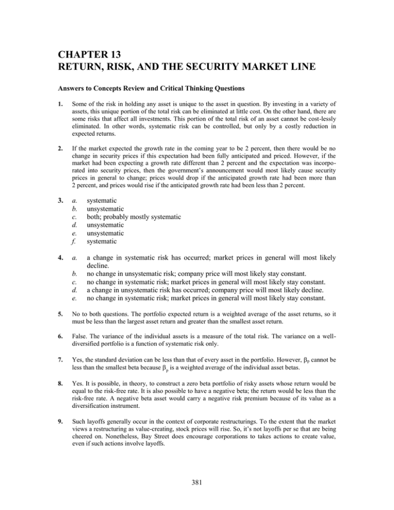
CHAPTER 13
RETURN, RISK, AND THE SECURITY MARKET LINE
Answers to Concepts Review and Critical Thinking Questions
1.
Some of the risk in holding any asset is unique to the asset in question. By investing in a variety of
assets, this unique portion of the total risk can be eliminated at little cost. On the other hand, there are
some risks that affect all investments. This portion of the total risk of an asset cannot be cost-lessly
eliminated. In other words, systematic risk can be controlled, but only by a costly reduction in
expected returns.
2.
If the market expected the growth rate in the coming year to be 2 percent, then there would be no
change in security prices if this expectation had been fully anticipated and priced. However, if the
market had been expecting a growth rate different than 2 percent and the expectation was incorporated into security prices, then the government’s announcement would most likely cause security
prices in general to change; prices would drop if the anticipated growth rate had been more than
2 percent, and prices would rise if the anticipated growth rate had been less than 2 percent.
3.
a.
b.
c.
d.
e.
f.
systematic
unsystematic
both; probably mostly systematic
unsystematic
unsystematic
systematic
4.
a.
a change in systematic risk has occurred; market prices in general will most likely
decline.
no change in unsystematic risk; company price will most likely stay constant.
no change in systematic risk; market prices in general will most likely stay constant.
a change in unsystematic risk has occurred; company price will most likely decline.
no change in systematic risk; market prices in general will most likely stay constant.
b.
c.
d.
e.
5.
No to both questions. The portfolio expected return is a weighted average of the asset returns, so it
must be less than the largest asset return and greater than the smallest asset return.
6.
False. The variance of the individual assets is a measure of the total risk. The variance on a welldiversified portfolio is a function of systematic risk only.
7.
Yes, the standard deviation can be less than that of every asset in the portfolio. However, p cannot be
less than the smallest beta because p is a weighted average of the individual asset betas.
8.
Yes. It is possible, in theory, to construct a zero beta portfolio of risky assets whose return would be
equal to the risk-free rate. It is also possible to have a negative beta; the return would be less than the
risk-free rate. A negative beta asset would carry a negative risk premium because of its value as a
diversification instrument.
9.
Such layoffs generally occur in the context of corporate restructurings. To the extent that the market
views a restructuring as value-creating, stock prices will rise. So, it’s not layoffs per se that are being
cheered on. Nonetheless, Bay Street does encourage corporations to takes actions to create value,
even if such actions involve layoffs.
381
10.
Earnings contain information about recent sales and costs. This information is useful for projecting
future growth rates and cash flows. Thus, unexpectedly low earnings often lead market participants
to reduce estimates of future growth rates and cash flows; price drops are the result. The reverse is
often true for unexpectedly high earnings.
Solutions to Questions and Problems
Basic
1.
total value = 90($35) + 70($25) = $4,900
weight1 = 90($35)/$4,900 = .6429 ; weight 2 = 70($25)/$4,900 = .3571
2.
E[Rp] = ($700/$3,100)(0.11) + ($2,400/$3,100)(0.18) = .1642
3.
E[Rp] = .50(.10) + .30(.18) + .20(.13) = .1300
4.
E[Rp] = .135 = .15wX + .10(1 – wX); wX = 0.70
investment in X = 0.70($10,000) = $7,000; investment in Y = (1 – 0.70)($10,000) = $3,000
5.
E[R] = .3(–.02) + .7(.34) = 23.2%
6.
E[R] = .4(–.05) + .5(.12) + .1(.25) = 6.5%
7.
E[RA] = .20(.06) + .60(.07) + .20(.11) = 7.60%
E[RB] = .20(–.2) + .60(.13) + .20(.33) = 10.40%
A2 =.20(.06–.0760)2 + .60(.07–.0760)2 + .20(.11–.0760)2 = .000304; A = [.000304]1/2 = .01744
B2 =.20(–.2–.1040)2 + .60(.13–.1040)2 + .20(.33–.1040)2 = .029104; B = [.029104]1/2 = .17060
8.
E[Rp] = .20(.05) + .70(.16) + .1(.35) = 15.70%
9.
a.
b.
10. a.
b.
boom: E[Rp] = (.07 + .15 + .33)/3 = .1833 ; bust: E[R p] = (.13 + .03 .06)/3 = .0333
E[Rp] = .60(.1833) + .40(.0333) = .1233
boom: E[Rp]=.20(.07) +.20(.15) + .60(.33) =.2420
bust: E[Rp] =.20(.13) +.20(.03) + .60(.06) = –.004
E[Rp] = .60(.2420) + .40(.004) = .1436
p2 = .60(.2420 – .1436)2 + .40(.004 – .1436)2 = .014524; p = [.014524]1/2 = .1205
boom:
E[Rp] = .30(.3) + .40(.45) + .30(.33) = .3690
good:
E[Rp] = .30(.12) + .40(.10) + .30(.15) = .1210
poor:
E[Rp] = .30(.01) + .40(–.15) + .30(–.05) = –.0720
bust:
E[Rp] = .30(–.06) + .40(–.30) + .30(–.09) = –.1650
E[Rp] = .20(.3690) + .40(.1210) + .30(–.0720) + .10(–.1650) = .0841
p2 = .20(.3690 – .0841)2 + .40(.1210 – .0841)2 + .30(–.0720 – .0841)2 + .10(–.1650 – .0841)2
p2 = .03029; p = [.03029]1/2 = .174
11. 2p = 0.0144 = (.4)2(.2)2 + .(.6)2y2 + 2(.4)(.6)(.2)(y)(.7)
= 0.0144 = .0064 + .36y2 + .0672y
.36y2 + .0672y – .008 = 0
While this equation can be solved using the quadratic formula, we only consider the positive root for
the standard deviation. We get: y = 0.0825 or 8.25%.
12. A $1 rise associated with a $0.60 drop suggests that the correlation between the returns for the two
stocks is –0.6. The portfolio variance becomes:
2p = (.25)2(.0225) + .(.75)2(.0121) + 2(.25)(.75)(.15)(.11)(-.6) = 0.0045
382
p = 0.0671.
When correlation = 0.5 we get:
2p = (.25)2(.0225) + .(.75)2(.0121) + 2(.25)(.75)(.15)(.11)(.5) = 0.0113
p = 0.1063.
When correlation = 1.0 we get:
2p = (.25)2(.0225) + .(.75)2(.0121) + 2(.25)(.75)(.15)(.11)(1) = 0.0144.
p = 0.12.
As the correlation between returns increases, so too do the variance and standard deviation of the
portfolio. The benefits of diversification are being reduced as the association between returns
increases.
13. p = .25(.9) + .20(1.4) + .15(1.1) + .40(1.8) = 1.39
14. p = 1.0 = 1/3(0) + 1/3(.8) + 1/3(X) ; X = 2.2
15. E[Ri] = .05 + (.14 – .05)(1.5) = .185
16. E[Ri] = .13 = .05 + .07i ; i = 1.14
17. E[Ri] = .10 = .06 + (E[RM] – .06)(.9) ; E[RM] = .1044
18. E[Ri] = .14 = Rf + (.11 – Rf)(1.6) ;
19. a.
b.
c.
d.
Rf = .060
E[Rp] = (.15 + .05)/2 = .10
p = 0.6 = xS(1.1) + (1 – xS)(0) ; xS = 0.6/1.1 = .5455 ; xRf = 1 – .5455 = .4545
E[Rp] = .09 = .15xS + .05(1 – xS) ; xS = .4; p = .4(1.1) + .6(0) = 0.44
p = 2.2 = xS(1.1) + (1 – xS)(0) ; xS = 2.2/1.1 = 2 ; xRf = 1 – 2 = –1
The portfolio is invested 200% in the stock and –100% in the risk-free asset. This represents
borrowing at the risk-free rate to buy more of the stock.
20. ßp = xW(1.4) + (1 – xW)(0) = 1.4xW
E[RW] = .17 = .04 + MRP(1.40) ; MRP = .13/1.4 = .0929
E[Rp] = .04 + .0929p ; slope of line = MRP = .0929 ; E[Rp] = .04 + .0929p = .04 + .13xW
xW
E[Rp]
ßp
xW
E[Rp]
p
0%
25
50
75
.0400
.0725
.1050
.1375
0
0.35
0.70
1.05
100%
125
150
.1700
.2025
.2350
1.40
1.75
2.10
21. E[Rii] = .06 + .075i
.17 > E[RY] = .06 + .075(1.45) = .1688;
Y plots above the SML and is undervalued.
reward-to-risk ratio Y = (.17 – .06) / 1.45 = .0759
.12 < E[RZ] = .06 + .075(0.85) = .1238;
Z plots below the SML and is overvalued.
reward-to-risk ratio Z = (.12 – .06) / .85 = .0706
22. [.17 – Rf]/1.45 = [.12 – Rf]/0.85 ;
Rf = .0492
Intermediate
23. For a portfolio that is equally invested in large-company stocks and long-term bonds:
return = (10.29% + 9.01%)/2 = 9.65%
For a portfolio that is equally invested in small stocks and Treasury bills:
383
return = (13.31% + 6.89%)/2 = 10.10%
24. (E[RA] – Rf)/A = (E[RB] – Rf)/ßB
RPA/A = RPB/B ; B/A = RPB/RPA
25. a.
b.
c.
boom: E[Rp] = .4(.20) + .4(.35) + .2(.60) = .34
normal: E[Rp] = .4(.15) + .4(.12) + .2(.05) = .118
bust:
E[Rp] = .4(.01) + .4(–.25) + .2(–.50) = –.196
E[Rp] = .2(.34) + .5(.118) + .3(–.196) = .0682
2p = .2(.34 – .0682)2 + .5(.118 – .0682)2 + .3(–.196 – .0682)2 = .036956
p = [.036956]1/2 = .1922
RPi = E[Rp] – Rf = .0682 – .038 = .0302
Approximate expected real return = .0682 – .035 = .0332
(1 + E[Ri]) = (1 + h)(1 + e[ri]) ;
Exact expected real return = e[ri] = [1.0682/1.035] – 1 = .0321
Approximate expected real risk premium = 0.0302 – 0.0350 = - 0.0048
Exact expected real risk premium = 1.0302 / 1.035 – 1 = - 0.0046
26. xA = $200,000 / $1,000,000 = .20;
xB = $250,000/$1,000,000 = .25 ; xC + xRf = 1 – xA – xB =
.55
p = 1.0 = xA(.7) + xB(1.1) + xC(1.6) + xRf(0); xC = .365625, invest .365625($1,000,000) = $365,625 in C.
xRf = 1 – .20 – .25 – .365625 = .184375
invest .184375($1,000,000) = $184,375 in the risk-free asset.
27. E[Rp] = .125 = wX(.28) + wY(.16) + (1 – wX – wY)(.07)
p = .8 = wX(1.6) + wY(1.2) + (1 – wX – wY)(0)
solving these two equations in two unknowns gives wX = –0.05555555 wY = 0.74074047
wR = 0.3148148
amount of stock X to sell short = –0.05555555($100,000) = $5,555.55
28. E[RI] = .2(.09) + .6(.42) + .2(.26) = .322 ; .322 = .04 + .10I , I = 2.82
I2 = .2(.09 – .322)2 + .6(.42 – .322)2 + .2(.26 – .322)2 = .017296;
I = [.017296]1/2 = .1315
E[RII] = .2(–.30) + .6(.12) + .2(.44) = .10 ; .10 = .04 + .10II , II = 0.60
II2 = .2(–.30 – .10)2 + .6(.12 – .10)2 + .2(.44 – .10)2 = .05536;
II = [.05536]1/2 = .2353
Although stock II has more total risk than I, it has much less systematic risk, since its beta is much
smaller than I’s. Thus, I has more systematic risk, and II has more unsystematic and more total risk.
Since unsystematic risk can be diversified away, I is actually the “riskier” stock despite the lack of
volatility in its returns. Stock I will have a higher risk premium and a greater expected return.
29. E[RPete Corp.] = .20 = Rf + 1.3(RM – Rf);
.20 = Rf + 1.3RM – 1.3Rf = 1.3RM – .3Rf;
Rf = (1.3RM – .20)/.3
E[RRepete Co.] = .14 = Rf + .8(RM – Rf)
.14 = Rf + .8(RM – Rf) = Rf + .8RM – .8Rf
RM = (.14 – .2Rf)/.8 = .175 – .25Rf
Rf = [1.3(.175 – .25Rf) – .20]/.3
.625Rf = .0275
Rf = .044
.20 = .044 + 1.3(RM – .044); RM = .164
.14 = .044 + .8(RM – .044);
384
RM = .164