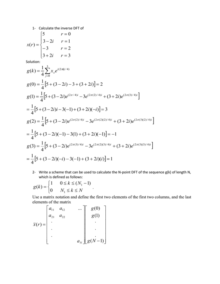
1- Calculate the inverse DFT of
5
 3  2i

x(r )  
 3

 3  2i
r 0
r 1
r2
r 3
Solution:
1 3
g (k )   x x e i ( 2kj / 4)
4 j 0
1
g (0)  5  (3  2i )  3  (3  2i )  2
4
1
g (1)  5  (3  2i )e( 2 / 4)i  3e( 2 ( 2) / 4)i  (3  2i)e( 2 (3) / 4)i
4
1
 5  (3  2i)i  3(1)  (3  2i)( i )  3
4
1
g (2)  5  (3  2i)e ( 2 ( 2) / 4)i  3e ( 2 ( 2)( 2) / 4)i  (3  2i)e ( 2 (3)( 2) / 4)i
4
1
 5  (3  2i)( 1)  3(1)  (3  2i)( 1)  1
4
1
g (3)  5  (3  2i)e ( 2 (3) / 4)i  3e ( 2 ( 2)( 3) / 4)i  (3  2i )e ( 2 (3)( 3) / 4)i
4
1
 5  (3  2i)( i)  3(1)  (3  2i)(i)  1
4






2- Write a scheme that can be used to calculate the N-point DFT of the sequence g(k) of length N,
which is defined as follows:
1
g (k )  
0
0  k  ( N1  1)
N1  k  N
.
Use a matrix notation and define the first two elements of the first two columns, and the last
elements of the matrix
 a11
a
 21
.
x (r )  
.

 .

a12
a22
...   g (0) 
  g (1) 


.




.


.



a N   g ( N  1)
N1 1
N 1
x (r )   e i ( 2kr / N ) g ( k )   e i ( 2kr / N ) g ( k ) (1) 
k 0
k 0
N 1
e
i ( 2kr / N ) g ( k )
(0)
k  N1
N 1
  e i ( 2kr / N )
k 0
1
 x1  1
 x  1 e  2 / N i
 2  
 .  .
 .   .

 
.

 .
 xN1 1  1
...
 1
 
 1
 . 
 . 
 
 1
  2 )( N1 1)( N1 1) / N i  1
e
  
1


2
, write a scheme that can be used to find  for any x in[0,1] at any time
x
t
t  0 given that if (0, t )  (1, t )  0 and  ( x,0)  1.0 . Discuss different ways that can be
3- If
used to improve the accuracy.
Divide the region between 0 and 1 in to N intervals such that
xi  i / N , for i=0..N.
Now divide the region between 0 and T, where T is any time when a final solution is sought, in to M
intervals such that
t j  j / N , for j=0..M.
Start with the two pint formula to write
 i 1, j   i ,i
2
 i , j 1   i , j
x
t
Where x  1 / N and t  1/ M . Rearrange the terms to get
t
t
 i , j 1 
 i 1, j  (1 
) i , j for i=0,..,N, j=0,..,M.
2x
2x
We can make increase N and/or M. We can also use a three point formula after j=1, or the five point
formula after j=3.
4- Use a Galerkin method to solve the one dimensional Poisson equation
 ( x)  1  0 between x=0 and x=1 with  ( 1)  1 and (3)  2 .
Let x=4y-1, then y is in [0,1] for x in [-1,3] and dx=4dy.
The equation then becomes:  ( y )  16
Let  
3
c
n 0
Then   
n
yn
3
 nc
n 1
n
y n1
N
   n(n  1)cn y n2
n2
The boundary conditions:
(0)  c0  1
(1)  1  c1  c2  c3  ..  2  c1  c2  c3  ..  1
3
1
1
n 2
0
0
 n(n  1)cn  y k 2 y n2 dy  16 y k dy for k=2,..,N. There are N-2 equations here and 1 from
the BC, which make it N-14 eqns and N-1 unknowns.
Take home component:
The position of a particle at different times, between t=0 and t=1, is given in the table below. If
the particle has an acceleration of -8/3 m/s2 at t=0, and we know that acceleration is a linear
function of time,
a- Find the velocity of the particle accurate to t 2 everywhere at the nodes.
b-Use cubic spline interpolation to approximate the position at any time t, then find the
velocity at the nodes and compare your results to part a.
t
x(t)
0
5
0.1 5.19
0.2 5.35
0.3 5.48
0.4 5.58
0.5 5.66
0.6 5.71
0.7 5.73
0.8 5.72
0.9 5.68
1 5.61
f i
f i1  f i1
 Ot 2
2t
(1.1)
f i1  f i1  2tf i,
(1.2)
f i1  f i1  2tf i
(1.3)
f i 
f i 1  f i 1
 Ot 2
2t
( 2)
First use equation (2) to find vi, i=1, .., 9. Next use equation (1.2) to find f 0 . Now use (1.1) to find f i for
f i1  f i1
to find the slope and then use
t
f i1  f i mti to find f 9 and f 10 . Now use (1.3) to find f 10 . v is accurate to order of t 2 everywhere.
i=1,..,9. Since f (t ) is a linear function of time use m 