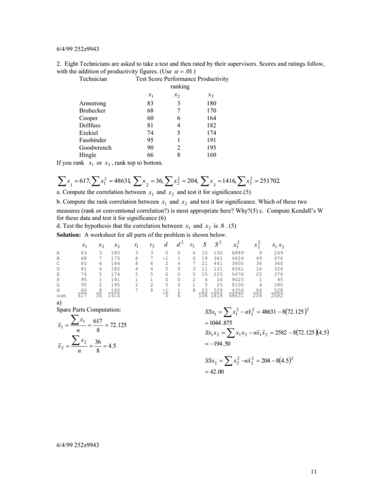
6/4/99 252z9943
2. Eight Technicians are asked to take a test and then rated by their supervisors. Scores and ratings follow,
with the addition of productivity figures. (Use   .01 )
Technician
Test Score Performance Productivity
ranking
x1
x2
x3
Armstrong
83
3
180
Brubecker
68
7
170
Cooper
60
6
164
Dollfuss
81
4
182
Ezekiel
74
5
174
Fassbinder
95
1
191
Goodwrench
90
2
195
Hingle
66
8
160
If you rank x1 or x3 , rank top to bottom.
x
1
 617,
x
2
1
 48631,
x
2
 36,
x
2
2
 204,
x
3
 1416,
x
2
3
 251702.
a. Compute the correlation between x1 and x 2 and test it for significance.(5)
b. Compute the rank correlation between x1 and x 2 and test it for significance. Which of these two
measures (rank or conventional correlation?) is most appropriate here? Why?(5) c. Compute Kendall’s W
for these data and test it for significance (6)
d. Test the hypothesis that the correlation between x1 and x 2 is .8 . (5)
Solution: A worksheet for all parts of the problem is shown below.
x1
A
B
C
D
E
F
G
H
sum
x2
83
68
60
81
74
95
90
66
617
3
7
6
4
5
1
2
8
36
x3
r1
r2
d
d2
180
170
164
182
174
191
195
160
1416
3
6
8
4
5
1
2
7
3
7
6
4
5
1
2
8
0
-1
2
0
0
0
0
-1
0
0
1
4
0
0
0
0
1
6
a)
Spare Parts Computation:
x1 
x2
x
1
n
x

n
2

617
 72 .125
8
36

 4.5
8
r3
4
6
7
3
5
2
1
8
S
S2
10 100
19 361
21 441
11 121
15 225
4
16
5
25
23 529
108 1818
SSx1 
x12
x 22
x1 x 2
6889
4624
3600
6561
5476
9025
8100
4356
48631
9
49
36
16
25
1
4
64
204
249
476
360
324
370
95
180
528
2582
x
 nx12  48631  872 .125 2
2
1
 1044 .875
Sx1 x 2 
x x
1 2
 nx1 x 2  2582  872 .125 4.5
 194 .50
SSx2 
x
2
2
nx 22  204  84.52
 42 .00
6/4/99 252z9943
11
The simple sample correlation coefficient is r 
 XY  nXY
 X  nX  Y
2
 XY  nXY 
, so using x

 X  nX  Y  nY 
2
2
 nY 2
2
R
2
2
2
194 .50

1044 .875 42 .00
2
2
2
in place of y , we get r  
square root of
 194 .50 2
1044 .875 42 .00 
 .9285 . From the outline, if we want to test H 0 : xy  0 against H1 : xy  0 and
x and y are normally distributed, we use t n  2  
r
1 r
n2
.9285

1   .9285 
82
2
6
 3.707 ,
 6.15 . Since t .005
2
we reject H 0 .
b) Remember that you were advised to rank x1 and x3 top to bottom. This is not the usual way of doing
things, but makes sense in this case since x 2 already has the best as 1. Remember that d  r1  r2 ,and then
rs  1 
 d  1  66  0.9285 . If we want a 2-sided test at the 99% confidence level of
nn  1
88  1
2
6
2
2
H 0 :   0 , compare rs with the 0.5% value from the Pearson’s rank correlation coefficient table. Since
the table value is .7450, reject the null hypothesis. We conclude that the rank correlation is significant.
c) Following the process in the outline, compute S 
SR 
n  1c  108
 SR
 13 .5 . From this Kendall’s W 
2
 
 n SR  1818  813.52  360 , where
S
8
n
3
n


360
 .9523 . If H 0 is
8
disagreement, S can be checked against a table for this test. But n is too large for the table, so use
S
 2n 1 
 k n  1W  37 .9523   20 . This has the  2 distribution with n  1  7 degrees of
1 knn  1
12
2
1 k2
12
1 32
12
8
3

freedom. Since  .2017   18.4753 is below our  2 , reject H 0 .
d) I don’t believe that anyone did this section. The outline says “ We need to use Fisher's z-transformation.
1  1  0 
1 1 r 
 and a standard deviation of
Let ~
z  ln 
 . This has an approximate mean of  z  ln 
2  1   0 
2  1 r 
~
n 2 
z  z
1

, so that t
.“
sz 
sz
n3
12
6/10/99 252z9943
3. Samples of demand for four types of sailboat sold by your firm are as follows:
West Coast East Coast Total
Pirates Revenge
74
146
220
Jolly Roger
54
110
164
Bluebeard’s Treasure
46
100
146
Ahab’s Quest
50
120
170
Total
224
476
700
Do all tests at the 95% confidence level.
a. Management had initially assumed that the proportion of total sales of “Pirates Revenge” would
be at most 30% of sales. Test this. (3)
b. Test the hypothesis that sales of the “Pirates Revenge” are the same proportion of sales on both
the East and West Coast (4)
c. Test the hypothesis that sales on the West Coast follow a uniform distribution (i.e. that each
model is the same proportion of West Coast sales) (5)
d. Test the hypothesis that the proportions of each boat sold are the same on both coasts. (5)
Solution:
a) Table 3 says the following:
Interval for
Confidence
Hypotheses
Test Ratio
Critical Value
Interval
pcv  p0  z 2 p
Proportion
p  p0
H 0 : p  p0
p  p  z 2 s p
z
p
H1 : p  p0
p0 q0
pq
p 
sp 
n
n

p  1 p
H 0 : p  .30
If we check the original data, total sales of “Pirates Revenge” were 220 Out of 700, or

H 1 : p  .30
p  p 0 .3143  .30 .0143


 .8256 . We reject
p  .3143. Thus, if we use the test ratio method z 
p
.30 .70  .01732
H 0 if it is greater than z .05
700
 1.645 . It is not so we do not reject H 0 .
b) From Table 3 again:
Interval for
Confidence
Interval
p  p  z 2 sp
Difference
between
p  p1  p 2
proportions
p1q1 p2 q 2
q  1 p
sp 

n1
n2
Hypotheses
Test Ratio
H 0 : p  p 0
z
H 1 : p  p 0
p 0  p 01  p 02
or p 0  0
p  p 0
 p
If p  0
 p 
p01q 01 p02 q 02

n1
n2
Or use
Critical Value
pcv  p0  z 2  p
If p0  0
 p 
p0 
p0 q 0  1 n1 
1
n2

n1 p1  n2 p2
n1  n2
s p
H 0 : p  0 H 0 : p1  p 2
Our Hypotheses are 
or 
where p  p1  p2 . If we use the test ratio method, we
H 1 : p  0
H 1 : p1  p 2
220
146
74
 .3143 , p1 
 .3067 . So p  p1  p 2
 .3304 and p 2 
need to find p 0 
700
476
224
 3304  .3067  .0237 .
6/10/99 252z9943
13


p 0 q 0  1  1   .3143 .6857  1
1
.
n2 
224
476  .00141  .036145
 n1
p  p 0
.0237
z

 6.2815 . Since z .025  1.960 do not reject H 0 .
 p
.036145
 p 
c) H 0 : Uniform .
So
Since O sums to 224 and there are 4 models, divide 224 by 4 to get 56. The actual
comparison can be done by either summing
E  O  2
E
O
E
E O
E  O2
74
54
46
50
224
56
56
56
56
224
-18
2
10
6
0
324
4
100
36
E  O2
or by summing
E  O  2
E
5.78571
0.07143
1.78571
0.64286
8.28571
O2
and subtracting n .
E
O2
E
97.7857
52.0714
37.7857
44.6429
232.2857
O2
 n  232 .2857  224  8.2857 . Since there are 4 items in
E
E

the comparison and we have used the data to estimate 1 parameter df  4  1  3 and  .2053  7.8147 , we
So  2 

 8.28571 or  2 

reject H 0 . The Kolmogorov-Smirnov method could also be used for this problem.
d) H 0 : Homogeneity . The proportions in rows, p r , are used with column totals to get the items in E .
Note that row sums in E are the same as in O .
O
sum
pr
E
sum
pr
74
146
220
.3142857
70 .40
149 .60
220
.3142857
54
46
110
100
164
146
.2342857
.2085714
52 .48
46 .72
111 .52
99 .28
164
146
.2342857
.2085714
50 120
sum 224 576
170
700
.2428571
1.000000
54 .40 115 .60 170
sum 224 .00 576 .00 700
.2428571
1.000000
The actual comparison can be done by either summing
So  2 
E O
O
E
74
54
46
50
146
110
100
120
700
70.40
52.48
46.72
54.40
149.60
111.52
99.28
115.60
700.00

E  O2
E
do not reject H 0 .
-3.60000
-1.52000
0.72000
4.40000
3.60001
1.52000
-0.72000
-4.40000
0.00000
 0.87513 or  2 
E  O2
12.9600
2.3104
0.5184
19.3600
12.9600
2.3104
0.5184
19.3600

E  O  2
E
or by summing
E  O  2
E
0.184091
0.044024
0.011096
0.355883
0.086631
0.020717
0.005222
0.167474
0.87513
DF  r  1c  1
 31  3
O2
and subtracting n .
E
O2
E
77.784
55.564
45.291
45.956
142.487
108.501
100.725
124.567
700.875
O2

 n  700 .875  700  0.875 . Since  .2053  7.8147 , we
E
14
6/10/99 252z9943
4. Data on passengers (in thousands), advertising (in $thousands) and (National income in $trillions)
appears below. (Use   .05 )
x 3 y (2) (This must be done correctly
pass
adv
inc
season
a) Compute

y
15
17
13
23
x1
10
12
8
17
x2
2.40
2.72
2.08
3.68
x3
1
1
1
1
to get full credit for b.)
b) Compute a simple regression of passengers against
National income. (6)
c) Compute R 2 (4)
d) Compute s e (3)
16
10
2.56
1
e) Compute s b2 ( the std deviation of the coefficient
21
14
20
26
18
17
18
23
15
16
y  272 ,
15
3.36
0
10
2.24
0
14
3.20
0
19
3.84
0
10
2.72
0
11
2.07
0
13
2.33
0
16
2.98
0
10
1.94
1
12
2.17
1
2
y  5128 ,
x  187,


 x y  3549 ,  x
1

2y
1
 759 .090 ,
of National Income) and do a confidence interval for
 2 .(3)
f) Do a confidence interval for Passengers, when
income is $4.10 billion. (3) At what income will
this interval be smallest? (1)
x
2
1
x x
1 2
 2469,
x
2
 40.29,
x
2
2
 113.339,
 525 .38 and n  15 . You do not need all of these.
Solution:
x 3 y  115   117   113   123   116   021  014   020   026   018 
a)

017   018   023  115   116   115
b) Spare Parts Computation:
x2 
y
x
2
n

SSx2 
40 .29
 2.6860
15
2
2
 nx 22  113 .339  152.686 2
 5.11975
 y  272  18.1333
n
x
Sx2 y 
x
2 y  nx 2 y
 759 .090  152.686 18 ..1333 
 28 .4979
15
SSy 
y
2
 ny  5128  1518 .1333 2
2
 195 .733  TSS
It seems reasonable to use the notation b2 instead of b1 .
b2 
Sx 2 y

SSx2
 x y  nx
 x  nx
2
2y
2
2
2

28 .4979
 5.5663
5.11975
b0  y  b2 x  18.1333  5.5663 2.686  3.1823
Yˆ  b0  b2 x 2 becomes Yˆ  3.1823 5.5663x 2 .
RSS 158 .6279
 x y  nx y   5.5663 28.4979   158 .6279 R  TSS

 0.8104 or
195 .733
 x y  nx y 
Sx y 
29.4979 
( 0  R  1 always!)



 .8104
SSx SSy  x  nx  y  ny  5.11975 195 .733 
c) RSS  b2 Sx 2 y  b2
2
2
2
2
R
2
2
2
2
2
2
2
2
2
2
2
2
2
2
15
6/10/99 252z9943
s e2 
d) ESS  TSS  RSS  195 .733  158 .627  37.106
formulas for s e2 see previous exam. s e  2.8543  1.6895
e) s b22 
s e2

SSx2

s e2
x 22
 nx 22


2.8543
 0.55751
5.11975
ESS 37 .106

 2.8543 or For other
n2
13
( s e2 is always positive!)
sb2  0.55751  0.7467
so
 2  b2  tsb2  5.5663 2.1600.7467  5.57  1.61
f) .
If Yˆ  3.1823 5.5663x 2 and x 20  4.10 , then Yˆ0  3.1823 5.56634.10  26.004
From the regression formula handout  Y0
1
So sY2ˆ  s e2  
 n
0

1
 Yˆ0  t sYˆ , where sY2ˆ  s e2  
n

X 0  X 2
 X
x2  x2 2 
 1 4.10  2.686 2 
 
  1.49525



2
.
8543
 15

5
.
11975
 x22  nx22 


2
 nX 2





0
s y0  1.49525  1.2228 .
So  Y0  Yˆ0  t sYˆ  26 .004  2.160 1.49525   26 .0  3.2 . This interval will be smallest when income
is $2.686 billion.
18
6/10/99 252zz9943
5. Data from problem 4 is repeated below. (Use   .01 )
y  272 ,
y 2  5128 ,
x  187,
x12  2469,


 x y  3549 ,  x
1

2y
1
 759 .090 ,

x x
1 2
x
2
 40.29,
x
 113.339,
2
2
 525 .38 and n  15 .
a. Do a multiple regression of passengers against advertising and National Income. (12)
b. Compute R 2 and R 2 adjusted for degrees of freedom for both this and the previous problem. Compare
the values of R 2 adjusted between this and the previous problem. Use an F test to compare R 2 here with
the R 2 from the previous problem.(5)
c. Compute the regression sum of squares and use it in an F test to test the usefulness of this regression. (5)
d. Use your regression to predict the number of passengers when we spend $13 (thousand) on advertising
and National Income is $3.5 (trillion).(2)
e. The regression on the previous page was run with the command
MTW > regress C1 on 1 C3;
SUBC > dw.
As a result, the last line of the regression read
Durbin-Watson statistic = 0.71
Solution: a) First, we compute Y  18 .1333 , X 1 
187
 12.4667 and X 2  2.6860 . Second, we compute
15
 X Y  3549 ,  X Y  759 .090 ,  Y  5128 ,  X  2469 ,  X  113 .339 and
 X X  525 .38 . Third, we compute our spare parts SSy   Y  nY  195 .733 ,
Sx y   X Y  nX Y  2469  1512.4667 18.1333   158 .067 , Sx y   X Y  nX Y
 759 .09  152.6860 18.1333   28 .4979 , SSx1   X 12  nX 12  2469  1512.46672  137.733 ,
SSx   X  nX  5.11975 and Sx x   X X  nX X  525 .38  1512 .4667 2.6860 
2
1
2
1
2
2
2
2
1
2
2
1
2
1
1
2
2
2
2
2
1 2
1
2
1
2
2
2
 23 .0979 . (Note that some of these were computed for the last problem.) Fourth, we substitute these
numbers into the Simplified Normal Equations:
X 1Y  nX 1Y  b1
X 12  nX 12  b2
X 1 X 2  nX 1 X 2


 X Y  nX Y  b  X X
2
which are
2
1
1
2
 
 nX X   b  X
1
2
2
2
2

 nX  ,
2
2
158 .067  137 .733 b1  23 .0979 b2
28 .4979  23 .0979 b1  5.11975 b2
and solve them as two equations in two unknowns for b1 and b2 . We do this by multiplying the second
equation by 4.5115, which is 23.0979 divided by 5.11975 so that the two equations become
158 .067  137 .733 b1  23 .0979 b2
, we then subtract the second equation from
128 .569  104 .207 b1  23 .0979 b2
the first to get 29.598  33.526 b1 , so that b1  0.8799 . The first of the two normal equations can now be
rearranged to get 23.0979 b2  128 .569  104 .207 0.8799  , which gives us b2  1.5963 . Finally we get b0
by solving b0  Y  b1 X 1  b2 X 2  18 .1333  0.8799 12 .4667   1.5963 2.6860   2.8762 . Thus our
equation is Yˆ  b0  b1 X 1  b2 X 2  2.8762  0.8799X 1  1.5963X 2
b) The coefficient of determination is R 2 

b1
 X Y  nX Y  b  X Y  nX Y 
 Y  nY
0.8799 158 .067   1.5963 28 .4979   .9430
195 .7333
1
1
2
2
2
2
2
. (The standard error is
19
6/10/99 252zz9943
s e2
Y

2
 nY 2  b1
 X Y  nX Y  b  X Y  nX Y   Y

1
1
2
2
n3
need it yet.) Our results can be summarized below as:
n
R2
.8104
15
.9430
15
2
2

 nY 2 1  R 2
n3
 , but we don’t
R2
.7958
.9335
k
1
2
R 2 , which is R 2 adjusted for degrees of freedom, has the formula R 2 
n  1R 2  k , where
k is the
n  k 1
number of independent variables. R 2 adjusted for degrees of freedom seems to show that our second
regression is better.
Y 2  nY 2  195 .733 . For the
The easiest way to do the F test and have it look right is to note that

regression with one independent variable the regression sum of squares is
R2
Y 2  nY 2  .8104 195 .733   158 .622 . For the regression with two independent variables the


regression sum of squares is R 2
 Y
2

 nY 2  .9430 195 .733   184 .576 . The difference between these
is 25.954. the remaining unexplained variation is 195.733 –184.576 = 11.157. the ANOVA table is
Source
SS
DF
MS
F
F.01
158.622
1
158.622
X2
X1
25.954
1
25.954
27.9105
1
F12
 9.33
11.157
12
0.9299
Error
195.733
14
Total
Since our computed F is larger than the table F , we reject our null hypothesis that X 1 has no effect.
c) We computed the regression sum of squares in the previous section.
Source
SS
DF
MS
F
F.01
184.576
2
92.288
99.245
X1 , X 2
F 2  6.93
12
11.157
12
0.9299
Error
195.733
14
Total
Since our computed F is larger than the table F , we reject our null hypothesis that X 1 and X 2 do not
explain Y .
d) Yˆ  b0  b1 X 1  b2 X 2  2.8762  0.8799X 1  1.5963X 2  2.8762  0.8799 13  1.5963 3.5 =11.103.
e) A Durbin-Watson Test is a test for autocorrelation. For   .01 , k  2 and n  15 , the test table gives
d L  .70 and d U  .1.25 .According to the text, the null hypothesis is ‘No Autocorrelation’ and our
rejection region is d  d L, or 4  d   d L, . We really should use the   .005 value for d L , but a
2
2
check of the   .05 table leaves us sure that it is below .70. thus the D-W statistic of 0.71 is not in the
rejection region. Check the examples to see that it could be in the “possibly significant” region.
20
6/14/99 252zz9943
6.(Watch it!) Three methods are used to train candidates for the FAA pilots exam. Scores for trainees are
shown below classified by method.
Method
a. Assume that the data is normal and compare the means
Video
Audio
for the first two methods (Assume unequal variances) (5)
Cassette Cassette Classroom
b. Do the same for all three methods (You may assume
72
73
68
equal variances now) (7)
86
75
83
80
60
50
c. Test column 1 to see if it has the normal distribution (5)
91
52
91
46
84
84
68
76
77
75
94
81
92
90
72
86
80
91
46
68
75
 x1

Note: For the first column:  x1  x1
 0.14 0.82 0.41 1.16  1.91  0.41 0.07
 s1
Note:
x
1
 518,
x
 39626,
2
1
x
3
 810,
x
2
3
 67240.
Note: In spite of the words “Watch it!, ” many people assumed that this was identical to a problem
with similar data on an earlier exam. You have to read the question before answering it!
x 2  420 ,
x 22  30090 , n3  10
Solution: Note: n1  7, n 2  6,


a) Assume unequal variances. From Table 3 of the Syllabus Supplement:
Interval for
Confidence
Hypotheses
Test Ratio
Interval
Difference
between Two
Means(
unknown,
variances
assumed
unequal)
H 0 :   0
H 1:   0
  d  t  sd
2
s12 s22

n1 n2
sd 
DF 
 s12 s22 
  
n

 1 n2 
2
  1   2
Same as
H 0: 1   2
2
s 22
n1
n1  1
d 0
sd
d cv   0  t  2 s d
H 1:  1   2
   
s12
t
Critical Value
2
if  0  0
n2
n2  1
Note: unequal variances like part a) here were strictly extra credit in Spring 2000!
x1 518
x12  nx12 39626  774 2
2
x1 

 74, s1 

 215 .6667 s1  14 .68559
n1
7
n1  1
6

x2 
x
n2

2

 H 0 : 1   2

 H 1 : 1   2
420
 70, s 22 
6
x
2
2
 nx 22
n2  1

s12 215 .6667

 30 .8095
n1
7
s 22 138 .0000

 23 .0000
n2
6
s12 s 22

 53 .8095
n1 n 2
30090  770 2
 138 .0000
5
sd 
s 2  11.74734 d  x1  x 2  4
s12 s 22

 53 .8095  7.3355
n1 n 2
21
6/14/99 252zz9943
DF 
 s12 s 22 



 n1 n 2 


2
2
2
 s12 
 s 22 
 
 
 n1 
 n2 
 
 

n1  1
n2 1

53 .8095 2
30 .8095 2  23 .0000 2
6
 10 .9675 , so use 10 degrees of freedom.
5
t.10
025  2.228 , so, using a test ratio t 
d  0
40

 0.545 . Since this is between 2.228 , do not
sd
7.3355
reject H 0 or, using a critical value, d cv   0  t s d  0  2.228 7.3355   16 .387 . Since d  4 is
2
between these values, do not reject H 0 .
b) 1-way ANOVA
Method
x2
73
75
60
52
84
76
x1
72
86
80
91
46
68
75
.
518
Sum
.
+ 420
x3
68
83
50
91
84
77
94
81
92
90
+810
= 1748 
= 23  n
nj
7
+6
+ 10
x j
74
70
81
SS
39626
+ 30090
+ 67240
x 2j
5476
4900
6561
Note that x is not a sum, but is
SSB 

n j x2j
 x . SST 
n
 x
76  x
= 136956   xij2
 x
2
ij
 n x  136956  2376 2  4108 .
2
 n x  75476   64900   10 6561   2376 2  494 .
Source
Between (Methods)
2
SS
494
DF
2
MS
247
F
1.365
( SSW  SST  SSB  3614 )
F.05
F 2, 20  3.49 ns
H0
Column means equal
Within (Error)
3614
20
181
Total
4108
22
2, 20  3.49 , we cannot reject
Because our computed F is smaller than F.05
H0
22
6/14/99 252zz9943
c) H 0 : Normal
We use the Lilliefors method because we are testing for the Normal distribution, we
have a small sample and the population mean and variance are unknown. The column Fe is the cumulative
distribution computed from the Normal table. t or z is
x1  x1
, which was computed for you.
s1
t or z
O Cumulative O
Fo
Fe
D
1
1
.14286 -1.91
.0281
.1148
1
2
.28571 -0.41
.3409
.0552
1
3
.42857 -0.14
.4443
.0157
1
4
.57142
0.07
.5279
.0435
1
5
.71428
0.41
.6591
.0552
1
6
.85714
0.82
.7939
.0632
1
7
1.00000
1.16
.8770
.1230
7
From the Lilliefors Table, the critical value for a 95% confidence level is .300. Since the largest number in
D is not above this value, we do not reject H 0 .
x1
46
68
72
75
80
86
91
23
6/14/99 252zz9943
7. (Watch it!) Three methods are used to train candidates for the FAA pilots exam. Scores for trainees are
shown below classified by method.
Method
a. Using a sign test, check x3 to see if it has a median of 85. (4)
Video
Audio
Cassette Cassette Classroom
b. Repeat the test on x3 using a more powerful method. (5)
x1
72
86
80
91
46
68
75
x2
73
75
60
52
84
76
Solution:
x3 x 3  85
68 -17
83
-2
50 -35
91
6
84
-1
77
-8
94
9
81
-4
92
7
90
5
x3
68
83
50
91
84
77
94
81
92
90
c. Apply the Runs Test as follows:
Write down the numbers in x1 and x3 together in order.
Underneath the numbers write down A if the number comes from
x1 and C if it comes from x3 . You will have a sequence like AACACC
….. . In case of a tie remove both tying numbers from your test.
Do a runs test on the resulting sequence to see if the A’s and C’s
appear randomly.
Congratulations! You have just done a Wald-Wolfowitz Test for the
equality of means in two (nonnormal) samples. If the sequence is
random, the means are equal. (6)
r r (corrected)
9
92
210
105
5
1
17
78
8
3
36
6
4
4
T   23
T   32
pvalue  2 Px  6  2 Px  4  2.37695 
 .7539 .
If   .05, this p-value is above the significance
level and we do not reject H 0 .
b) To do a Wilcoxon Signed Rank Sum Test,
rank the differences from 85 and put the sign of
the difference next to these ranks. To check ,
nn  1
note that T    T   55 
. From
2
the table the 2 1 2 % critical value is 8, since
both Ts are above this value, do not reject H 0 .
a) H 0 :  85 . To do a sign test, note that there
are 6 numbers below 85 and 4 above. Using the
binomial table with n  10, p  .5,
c) The numbers written out in order are:
46 50 68 68 72 75 77 80 81 83 84 86 90 91 91 92 94

A C C A A A C A C C C A C C A C C
46 50 72 75 77 80 81 83 84 86 90 92 94
If we eliminate ties we get: 
A C A A C A C C C A C C C
The number of As is n1  5 and the number of Cs is n 2  7 and there are r  8 runs. If we look this up
in the table entitled “Critical Values of r for the Runs Test, ” we fine that the upper critical value is 11 and
the lower critical value is 3. Since 8 lies between these values we do not reject the null hypothesis of
randomness. Out final conclusion is that the means of the populations from which the two samples come are
equal.
24