Summary Statistics
When analysing practical sets of data, it is useful to be able to define a small number of
values that summarise the main features present. We will derive (i) representative values, (ii)
measures of spread and (iii) measures of skewness and other characteristics.
Representative Values
These are sometimes called measures of location or measures of central tendency.
1. Random Value
Given a set of data S = { x1, x2, … , xn }, we select a random number, say k, in the range 1 to
n and return the value xk. This method of generating a representative value is
straightforward, but it suffers from the fact that extreme values can occur and successive
values could vary considerably from one another.
2. Arithmetic Mean
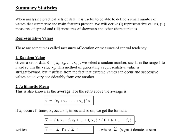
This is also known as the average. For the set S above the average is
x = {x1 + x2 + … + xn }/ n.
If x1 occurs f1 times, x2 occurs f2 times and so on, we get the formula
x = { f 1 x1 + f 2 x2 + … + f n xn } / { f 1 + f 2 + … + f n } ,
written
x =
 fx /  f
, where  (sigma) denotes a sum.
Example 1.
The data refers to the marks that students in a class obtained in an examination. Find the
average mark for the class. The first
point to note is that the marks are presented as Mark
Mid-Point Number
ranges, so we must be careful in our
of Range
of Students
interpretation of the ranges. All the intervals
xi
fi
f i xi
must be of equal rank and their must be no
gaps in the classification. In our case, we
0 - 19
10
2
20
interpret the range 0 - 19 to contain marks
21 - 39
30
6
180
greater than 0 and less than or equal to 20.
40 - 59
50
12
600
Thus, its mid-point is 10. The other intervals 60 - 79
70
25
1750
are interpreted accordingly.
80 - 99
90
5
450
Sum
50
3000
The arithmetic mean is x = 3000 / 50 = 60 marks.
Note that if weights of size fi are suspended
from a metre stick at the points xi, then the
average is the centre of gravity of the
distribution. Consequently, it is very sensitive
to outlying values.
x1
x2
f1
x
xn
fn
f2
Equally the population should be homogenous for the average to be meaningful. For
example, if we assume that the typical height of girls in a class is less than that of boys,
then the average height of all students is neither representative of the girls or the boys.
3. The Mode
Frequency
50
This is the value in the distribution that occurs
most frequently. By common agreement,
it is calculated from the histogram using linear
interpolation on the modal class.
13 20
25
13
The various similar triangles in the diagram
generate the common ratios. In our case,
the mode is
60 + 13 / 33 (20) = 67.8 marks.
20
12
6
2
20
5
40
60
80
40
60
80
100
4. The Median
Cumulative
50
This is the middle point of the distribution. It
is used heavily in educational applications. If
{ x1, x2, … , xn } are the marks of students in a
class, arranged in non-decreasing order, then 25.5
the median is the mark of the (n + 1)/2 student.
It is often calculated from the ogive or
cumulative frequency diagram. In our case,
the median is
60 + 5.5 / 25 (20) = 64.4 marks.
Frequency
20
100
Measures of Dispersion or Scattering
Example 2. The following distribution has the same
arithmetic mean as example 1, but the values are more
dispersed. This illustrates the point that an average
value on its own may not adequately describe a
statistical distributions.
To devise a formula that traps the degree to which a
distribution is concentrated about the average, we
consider the deviations of the values from the average.
If the distribution is concentrated around the mean,
then the deviations will be small, while if the distribution
is very scattered, then the deviations will be large.
The average of the squares of the deviations is called
the variance and this is used as a measure of dispersion.
The square root of the variance is called the standard
deviation and has the same units of measurement as
the original values and is the preferred measure of
dispersion in many applications.
Marks
x
Frequency
f
10
30
50
70
90
Sums
6
8
6
15
15
50
fx
60
240
300
1050
1350
3000
x6
x5
x4
x3
x2
x1
x
Variance & Standard Deviation
s2 = VAR[X] = Average of the Squared Deviations
= S f { Squared Deviations } / S f
= S f { xi - x } 2 / S f
= S f xi 2 / S f - x 2
, called the product moment formula.
s = Standard Deviation =  Variance
Example 1
f
x
2
10
6
30
12
50
25
70
5
90
50
fx
20
180
600
1750
450
3000
f x2
200
5400
30000
122500
40500
198600
VAR [X] = 198600 / 50 - (60) 2
= 372 marks2
Example 2
f
x
6
10
8
30
6
50
15
70
15
90
50
fx
60
240
300
1050
1350
3000
f x2
600
7200
15000
73500
121500
217800
VAR [X] = 217800 / 50 - (60)2
= 756 marks2
Other Summary Statistics
Skewness
An important attribute of a statistical distribution relates to its degree of symmetry. The
word “skew” means a tail, so that distributions that have a large tail of outlying values on the
right-hand-side are called positively skewed or skewed to the right. The notion of negative
skewness is defined similarly. A simple formula for skewness is
Skewness = ( Mean - Mode ) / Standard Deviation
which in the case of example 1 is:
Skewness = (60 - 67.8) / 19.287 = - 0.4044.
Coefficient of Variation
This formula was devised to standardise the arithmetic mean so that comparisons can be
drawn between different distributions.. However, it has not won universal acceptance.
Coefficient of Variation = Mean / standard Deviation.
Semi-Interquartile Range
Just as the median corresponds to the 0.50 point in a distribution, the quartiles Q 1, Q2, Q3
correspond to the 0.25, 0.50 and 0.75 points. An alternative measure of dispersion is
Semi-Interquartile Range = ( Q3 - Q1 ) / 2.
Geometric Mean
For data that is growing geometrically, such as economic data with a high inflation effect, an
alternative to the the arithmetic mean is preferred. It involves getting the root to the power
N = S f of a product of terms
Geometric Mean = N x1f1 x2 f2 … xk fk