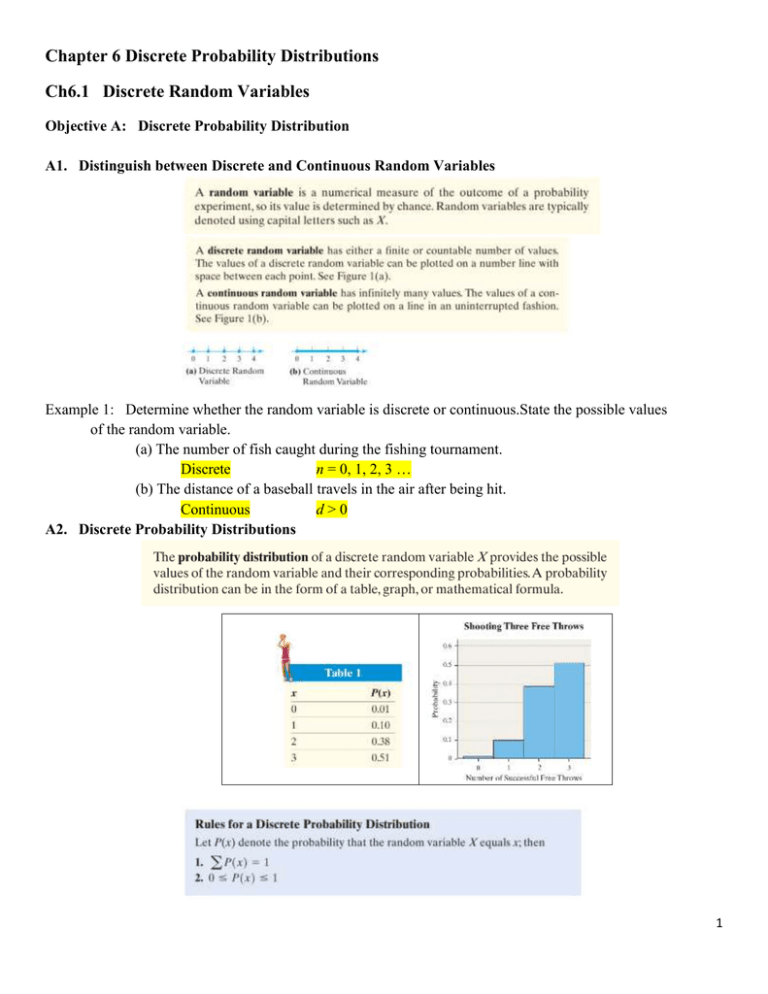
Chapter 6 Discrete Probability Distributions
Ch6.1 Discrete Random Variables
Objective A: Discrete Probability Distribution
A1. Distinguish between Discrete and Continuous Random Variables
Example 1: Determine whether the random variable is discrete or continuous.State the possible values
of the random variable.
(a) The number of fish caught during the fishing tournament.
Discrete
n = 0, 1, 2, 3 …
(b) The distance of a baseball travels in the air after being hit.
Continuous
d>0
A2. Discrete Probability Distributions
1
Example 1: Determine whether the distribution is a discrete probability distribution. If not, state why
 P(x)  0.73
 P(x) 1
Table (a)
Not a discrete probability distribution because it does not meet ∑ P (x) = 1.
Table (b)
It is a discrete probability distribution because it meets ∑ P (x) = 1
and each P(x) is between 0 and 1.
Example 2: (a) Determine the required value of the missing probability to make the distribution
a discrete probability distribution.
(a) The required value of the missing probability
P (x = 0) +P (x = 1) + P (x = 2) + P (x = 3) + P (x = 4) + P (x = 5) =1
0.30 + 0.15 + P (x = 2) + 0.20 + 0.15 + 0.05 = 1
P (x = 2) + 0.85 = 1
P(x = 2) = 1 – 0.85 = 0.15
2
(b) Draw a probability histogram.
P (x )
0.50
0.40
0.30
0.20
0.10
x
0
1
2
3
4
5
Objective B: The Mean and Standard Deviation of a Discrete Random Variable
3
Example 1: Find the mean, variance, and standard deviation of the discrete random variable x .
(a) Mean
x  [ x  P( x)]
x
0
1
2
3
4
(1)
x  P( x)
P( x)
0.073
0.117
0.258
0.322
0.230
(b) Variance --->
0 * (0.073) = 0
1 * (0.117) = 0.117
2 * (0.258) = 0.516
3 * (0.322) = 0.966
4 * (0.230) = 0.920
 x  [ x  P( x)]
 2.519
Use the definition formula
 x 2  [( x  x )2  P( x)]
Formula (2a) in the textbook
x  x
( x   x ) 2  P( x)
0.073
X*P(x)
0  (0.073)
0  2.519  2.519
(2.519) 2 (0.073)  0.463211353
1
0.117
1 (0.117)
1  2.519  1.519
(1.519) 2 (0.117)  0.269961237
2
0.258
2  (0.258)
(0.519) 2 (0.258)  0.069495138
3
4
0.322
0.230
3 (0.322)
4  (0.230)
2  2.519  0.519
3  2.519  0.481
4  2.519  1.481
x
0
P( x)
 x  [ x  P( x)]
 2.519
(0.481) 2 (0.322)  0.074498242
(1.481) 2 (0.230)  0.50447303
 x 2  [( x   x ) 2  P( x)]  1.381639
 x  1.381639  1.18
*Use StatCrunch to find the mean and standard deviation of the discrete random variable x in Example 1.
Steps: 1) Enter the data: X and P(X).
2) Click Stat → Calculators → Custom.
3) Choose X for Values in: and P(X) for Weights in:
4) Click Compute!
Objective C : Expected Value
The mean of a random variable is the expected value, E ( x)   x  P( x) , of the probability
experiment in the long run. In game theory x is positive for money gained and x is negative for
money lost.
4
Example 1:A life insurance company sells a $250,000 1-year term life insurance policy to a 20year-old male for $350. According to the National Vital Statistics Report, 56(9),
the probability that the male survives the year is 0.998734. Compute and interpret
the expected value of this policy to the insurance company.
Gain/Loss
Gain
Loss
x
+350
-249650
P(x)
0.998734
1-0.998734 = 0.001266
X * P (x)
350 * (0.998734) = 349.5569
-249650*(0.001266) = -316.0569
E( x)  [ x  P( x)]  33.5
In the long run, the insurance company will profit $ 33.50 per 20-year-old male.
Chapter 6.2 The Binomial Probability Distribution
Objective A : Criteria for a Binomial Probability Experiment
The binomial probability distribution is a discrete probability distribution that obtained from a
binomial experiment.
Example 1: Determine which of the following probability experiments represents a binomial
experiment. If the probability experiment is not a binomial experiment, state why.
(a) A random sample of 30 cars in a used car lot is obtained, and their mileages
recorded.
Not a binomial distribution because the mileage can have more than 2 outcomes.
(b) A poll of 1,200 registered voters is conducted in which the repondents are asked
whether they believe Congress should reform Social Security.
A binomial distribution because
– there are 2 outcomes.
(should or should not reform Social Security)
5
– fixed number of trials. (n = 1200)
– the trials are independent.
– we assume the probability of success is the same for
each trial of experiment.
Objective B : Binomial Formula
Let the random variable x be the number of successes in n trials of a binomial experiment.
Example 1: A binomial probability experiment is conducted with the given parameters.
Compute the probability of x successes in the n independent trials of the
experiment.
n  15, p  0.85, x  12 (Round to four decimal places as needed)
P (x)=𝑛 𝐶𝑥 𝑃 𝑥 (1 − 𝑝)𝑛−𝑥
P (x = 12) =15 𝐶12 (0.85) 12 (1 − 0.85) 15−12
= 455 (0.85) 12 (0.15)3≈ 0.2184
6
Example 2: (a) Use StatCrunch to compute a Binomial table of n  4 and p  0.65 .
First, state the possible values of the random variable x , then Open StatCrunch  select
Stat  Calculators  Binomial  Standard  Input n  4 and p  0.65  For P(x = 0),
select = in the inequality box  Input 0  Compute  Record the result  Repeat for
each x value 1, 2, 3 and 4 to complete the table.
x
0
1
2
3
4
P( x)
x
0
1
2
3
4
P( x)
0.01500625
0.111475
0.3105375
0.384475
0.17850625
(b) Use the Binomial table from part (a), find P ( x  2) .
P(x > 2) = 0.384475 + 0.17850625 = 0.56298125
(c) Use the Binomial table from part (a), find P(0  x  3) .
P(0  x  3) = 0.01500625 + 0.111475 + 0.3105375 = 0.43701875
Objective C : Binomial Table by StatCunch
Example 1: Use StatCrunch with Binomial Distribution to find P ( x  6) with n  12 and p  0.4 .
Open StatCrunch  select Stat  Calculators  Binomial  Standard  Input n = 12
and p = 0.4  For P(x ≤ 6), select  in the inequality box  Compute and record the
result. (If you need to include the graph, right click on image, select copy image, Paste
Special, then select Device Independent Bitmap)
7
Example 2 According to the American Lung Association, 90% of adult smokers started smoking
beforeturning 21 years old. Ten smokers 21 years old or older are randomly selected,
and thenumber of smokers who started smoking before 21 is recorded.
(a) Explain why this is a binomial experiment.
− There are 2 outcomes (smoke or not)
− The probability of success is the same for each trial of experiment
−The trials are independent
− Fixed numbers of trials n = 10
(b) Use StatCrunch to find the probability that exactly 8 of them started smoking before 21
years of age.
Open StatCrunch  Stat  Calculator  Binomial  Standard  Input n = 10 and p =
0.9  For P(x = 8), select = in the inequality box  Compute and record the result.
The probability that exactly 8 started smoking before 21 years of age is
P (x = 8) = 0.19371024
8
(c) Use StatCrunch to find the probability that at least 8 of them started smoking before 21
years of age.
Open StatCrunch  Stat  Calculator  Binomial  Standard  Input n = 10 and
p = 0.9  For P(x ≥ 8) , select  in the inequality box  Compute and record the result.
P ( x = 8 or more) = P (x ≥ 8) = 0.92980917
(d) Use StatCrunch to find the probability that between 7 and 9 of them, inclusive, started
smoking before 21years of age.
Open StatCrunch  Stat  Calculator  Binomial  Between  Input n = 10 and
p = 0.9  For P(7 ≤ x ≤ 9), Input 7 and 9 in the compound inequality box  Compute
and record the result.
P (7 ≤ X ≤ 9) = 0.63852636
9
Objective D : Mean and Standard Deviation of a Binomial Random Variable
Example 1: A binomial probability experiment is conducted with the given parameters.
Compute themean and standard deviation of the random variable x .
n9
p  0.8
𝜇𝑥 = n ∗ p = 9 * 0.8 = 7.2
𝜎𝑥 = √np(1- p)= √9(0.8)(1-0.8) = √9(0.8)(0.2) = 1.2
Example 2: According to the 2005 American Community Survey, 43% of women aged 18 to 24
wereenrolled in college in 2005.
(a)
For 500 randomly selected women ages 18 to 24 in 2005, compute the mean
and standarddeviation of the random variable x , the number of women who
were enrolled in college.
n  500,
p  0.43
𝜇𝑥 = n*p = 500 *0.43 = 215
𝜎𝑥 = √np (1-p) = √500(0.43)(1-0.43)
= √500(0.43)(0.57) ≈ 11.070
(b) Interpret the mean.
An average of 215 out of 500 randomly selected women aged 18 to 24 were enrolled in
college.
What role do p and n play in the shape of a binomial distribution? Study the textbook pg. 318-319.
In Other Words
Provided that np(1  p)  10, the interval   2 to   2 represent the “usual” observations. Observations
outside this interval may be considered unusual.
10