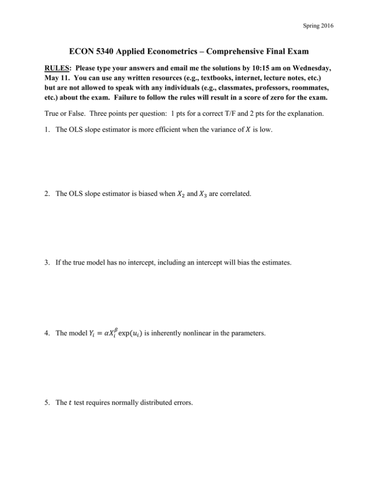
Spring 2016
ECON 5340 Applied Econometrics – Comprehensive Final Exam
RULES: Please type your answers and email me the solutions by 10:15 am on Wednesday,
May 11. You can use any written resources (e.g., textbooks, internet, lecture notes, etc.)
but are not allowed to speak with any individuals (e.g., classmates, professors, roommates,
etc.) about the exam. Failure to follow the rules will result in a score of zero for the exam.
True or False. Three points per question: 1 pts for a correct T/F and 2 pts for the explanation.
1. The OLS slope estimator is more efficient when the variance of 𝑋 is low.
2. The OLS slope estimator is biased when 𝑋2 and 𝑋3 are correlated.
3. If the true model has no intercept, including an intercept will bias the estimates.
𝛽
4. The model 𝑌𝑖 = 𝛼𝑋𝑖 exp⁡(𝑢𝑖 ) is inherently nonlinear in the parameters.
5. The 𝑡 test requires normally distributed errors.
Spring 2016
6. Measurement error in the dependent variable causes no bias in the estimated coefficients.
7. Heteroscedasticity biases the coefficients towards zero.
8. Severe multicollinearity will lead to inefficient OLS estimates.
9. If there is no heteroscedasticity in the population, then OLS and feasible GLS will be equal.
10. The Durbin Watson test is valid with lagged dependent variables.
Spring 2016
#11. (20 pts) Derive the OLS estimator for a regression model with one explanatory variable and
an intercept. Check the second-order conditions. Now consider the sample:⁡⁡𝑌 = (2,0,2,4)′;
𝑋 = (3,1,2,2)′. Find the estimated intercept and slope. Draw a figure showing the data points,
sample regression line, and all the residuals. Does the regression line go through the sample
means? Do the residuals sum to zero? Calculate the⁡𝑅 2 . Finally, provide an 𝐹⁡test for overall
goodness of fit. [The critical F for a 5% significance level is 𝐹𝑐 (1,2) =18.5.]
Spring 2016
#12. (50 pts) Consider the earnings model:
𝑊𝑎𝑔𝑒𝑖𝑡 = 𝛼𝑖 + 𝛽1 𝐴𝑔𝑒𝑖𝑡 ⁡+⁡𝛽2 𝐸𝑥𝑝𝑒𝑟𝑖𝑡 + 𝛽3 𝐸𝑑𝑢𝑐𝑖𝑡 + 𝑢𝑖𝑡 ,
(1)
where 𝑊𝑎𝑔𝑒 is the measured in dollars per hour, 𝐸𝑑𝑢𝑐 is the number of years of schooling,
𝐸𝑥𝑝𝑒𝑟 is the number of years of work experience, 𝑖 = 1, … , 𝑁 and 𝑡 = 1, … , 𝑇.
a) When is pooled OLS appropriate? When is fixed effects (FE) appropriate? When is random
effects (RE) appropriate? Propose a testing procedure to distinguish between the three models.
b) Consider the FE model. Provide an economic interpretation of the coefficients, including the
𝛼𝑖 estimates. Name three econometric issues that may affect the OLS estimates. Describe
how you would test for and resolve each issue.
Spring 2016
c) Assume a single cross section, 𝑖 = 1. How would you test for and correct for serial
correlation? In your answer, discuss the tradeoff between OLS and feasible GLS.
d) Assume a single time period, 𝑡 = 1. How would you test for and correct for
heteroscedasticity? In your answer, discuss the tradeoff between OLS and feasible GLS.
Spring 2016
e) Now consider a modification of equation (1) where there are only two wage categories, high
and low. Derive the expression for the probability of having a high wage and the probability
of having a low wage. Derive the marginal effect for education and describe how it differs
from⁡𝛽3. How does the pseudo-𝑅 2 differ from the traditional⁡𝑅 2 ?
Spring 2016
BONUS QUESTION. (5 pts) Consider the marginal effect, 𝛿𝑒𝑑𝑢𝑐,𝑖𝑡 , for education in problem
#12e. STATA provides standard errors for these marginal effects. Discuss the two sources of
uncertainty that drive the standard errors and any issues associated with their calculation.