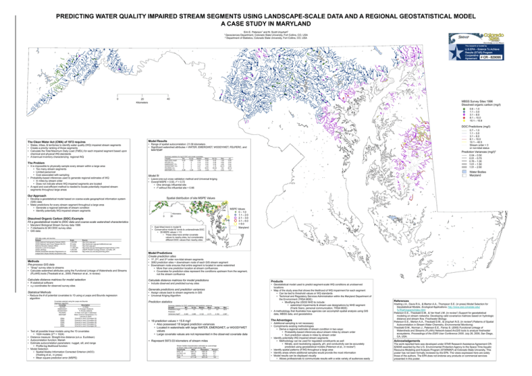
PREDICTING WATER QUALITY IMPAIRED STREAM SEGMENTS USING LANDSCAPE-SCALE DATA AND A REGIONAL GEOSTATISTICAL MODEL
A CASE STUDY IN MARYLAND
Erin E. Peterson1 and N. Scott Urquhart2
1 Geosciences Department, Colorado State University, Fort Collins, CO, USA
2 Department of Statistics, Colorado State University, Fort Collins, CO, USA
This research is funded by
U.S.EPA – Science To Achieve
Results (STAR) Program
Cooperative
Agreement # CR - 829095
0
40
20
Kilometers
MBSS Survey Sites 1996
Dissolved organic carbon (mg/l)
0.6 – 1.0
1.1 – 3.0
3.1 – 8.0
8.1 – 10.0
10.1 – 15.9
DOC Predictions (mg/l)
The Clean Water Act (CWA) of 1972 requires
• States, tribes, & territories to identify water quality (WQ) impaired stream segments
• Create a priority ranking of those segments
• Calculate the Total Maximum Daily Load (TMDL) for each impaired segment based upon
chemical and physical WQ standards
• A biannual inventory characterizing regional WQ
Model Results
• Range of spatial autocorrelation: 21.09 kilometers
• Significant watershed attributes = WATER, EMERGWET, WOODYWET, FELPERC, and
MINTEMP
Summary statistics for log10 DOC and model covariates.
Variable
Min
1st Qu.
Median
log10 DOC (mg/l)
-0.22
0.08
0.24
WATER (%)
0
0
0.16
EMERGWET (%)
0
0
0.13
WOODYWET (%)
0
0
0.27
FELPERC (%)
0
0
0.31
MINTEMP (°C)
-5.88
-3.06
-2.39
The Problem
• It is impossible to physically sample every stream within a large area
• Too many stream segments
• Limited personnel
• Cost associated with sampling
• Probability-based inferences used to generate regional estimates of WQ
• In miles by stream order
• Does not indicate where WQ impaired segments are located
• A rapid and cost-efficient method is needed to locate potentially impaired stream
segments throughout large areas
Mean
0.28
0.25
0.26
1.24
26.81
-2.49
3rd Qu.
0.43
0.28
0.35
1.15
55.26
-1.4
Max
1.20
4.64
4.85
22.01
100
0.03
Spatial distribution of site MSPE Values
0
MSPE Values
0 – 1.0
1.1 – 2.0
2.1 – 3.0
3.1 – 6.0
> 6.0
Maryland
30
Dissolved Organic Carbon (DOC) Example
Fit a geostatistical model to DOC data and coarse-scale watershed characteristics
Source
http://nhd.usgs.gov/
http://landcover.usgs.gov/natllandcover.asp
http://ned.usgs.gov/
http://www.epa.gov/wed/pages/ecoregions/level_iii.htm
USEPA Western Ecology Division, Corvallis, OR
http://www.ocs.orst.edu/prism/faq.phtml
σ2
0.25
0.44
0.44
3.28
36.14
1.47
• Leave-one-out cross validation method and Universal kriging
• Overall MSPE = 0.93, r2 = 0.72
• One strongly influential site
• r2 without the influential site = 0.66
Kilometers
Scale
1:250,000
30 meter
30 meter
1:7,500,000
1:250,000
4 kilometer
• East-West trend in model fit
• Conservative model fit: tends to underestimate DOC
• 35 MSPE values > 1.5
• These sites have similar covariate
values to nearby sites, but considerably
different DOC values than nearby sites
Model Predictions
Create prediction sites
• “Snap” survey sites to streams
• Calculate watershed attributes using the Functional Linkage of Watersheds and Streams
(FLoWS) tools (Theobald et al., 2005; Peterson et al., in review)
• 1st, 2nd, and 3rd order non-tidal stream segments
• 3083 prediction sites = downstream node of each GIS stream segment
• Downstream node ensures that entire segment is located in same watershed
• More than one prediction location at stream confluences
• Covariates for prediction sites represent the conditions upstream from the segment,
not the stream confluence
Calculate distance matrices for model selection
Calculate distance matrices for model predictions
Methods
Pre-process GIS data
• R statistical software
• x,y coordinates for observed survey sites
Products
• Include observed and predicted survey sites
Generate predictions and prediction variances
Statistical Methods
• Reduce the # of potential covariates to 10 using a Leaps and Bounds regression
algorithm
Covariates selected using the Leaps and Bounds
regression algorithm.
Description
Covariate
% Water
WATER
% Emergent Wetlands
EMERGWET
% Woody wetlands
WOODYWET
% Felsic rock type in watershed
FELPERC
Mean minimum temperature (°C)
MINTEMP
(January to April)
Omernik's Level 3 Ecoregion 64
ER64
Omernik's Level 3 Ecoregion 65
ER65
Omernik's Level 3 Ecoregion 66
ER66
Omernik's Level 3 Ecoregion 67
ER67
Omernik's Level 3 Ecoregion 69
ER69
• Test all possible linear models using the 10 covariates
• 1024 models (210 = 1024)
• Distance measure: Straight-line distance (a.k.a. Euclidean)
• Autocorrelation function: Mariah
• Estimate autocorrelation parameters: nugget, sill, and range
• Profile-log likelihood function
• Model Selection
• Spatial Akaike Information Corrected Criterion (AICC)
(Hoeting et al., in press)
• Mean square prediction error (MSPE)
0.04 – 0.50
0.51 – 0.75
0.76 – 1.00
1.01 – 1.50
1.51 – 2.60
Model fit
• Develop a geostatistical model based on coarse-scale geographical information system
(GIS) data
• Make predictions for every stream segment throughout a large area
• Generate a regional estimate of stream condition
• Identify potentially WQ impaired stream segments
GIS data, scale, and sources.
Dataset
USGS National Hydrography Dataset (NHD)
USGS National Land Cover Dataset (NLCD)
National Elevation Dataset (NED)
Omernik's Level III Ecoregion
USGS Lithology
PRISM (Parameter-elevation Regressions on
Independent Slopes Model) temperature data
Prediction Variances (mg/l)2
Water Bodies
Maryland
Our Approach
• Maryland Biological Stream Survey data 1996
• 7 interbasins & 343 DOC survey sites
• GIS data:
0.7 – 1.0
1.1 – 3.0
3.1 – 8.0
8.1 – 10.0
10.1 – 40.5
Stream order > 3
or non-tidal status
• Assign values back to stream segments in GIS
• Universal Kriging Algorithm
Prediction statistics
Summary statistics for DOC predictions and prediction variances.
Variable
Min
1st Qu.
Median
Mean
Predictions (mg/l)
0.8
1.5
1.9
2.7
Prediction
Variances (mg/l)2
0.049
0.095
0.122
0.171
3rd Qu.
3.0
Max
40.4
0.193
2.597
• 18 prediction values > 15.9 mg/l
• Also possessed 18 largest prediction variances
• Located in watersheds with large WATER, EMERGWET, or WOODYWET
values
• Large covariate values are not represented in the observed covariate data
• Represent 5973.03 kilometers of stream miles
Stream habitat characterization estimated as a percentage
of stream miles in DOC (mg/l) during 1996.
Thresholds
Miles
Kilometers
Percent
DOC < 5
3347.74
5387.67
90.2
5 ≤ DOC ≤ 8
248.67
400.19
6.7
DOC > 8
115.06
185.16
3.1
Total
3711.46
5973.03
100
• Geostatistical model used to predict segment-scale WQ conditions at unobserved
locations
• Map of the study area that shows the likelihood of WQ impairment for each segment
• Can be tied to threshold values or WQ standards
• Technical and Regulatory Services Administration within the Maryland Department of
the Environment (TRSA MDE)
• Modifying the USGS NHD to include:
• watershed impairments & stream-use designations by NHD segment
(Frank Siano, personal communication, TRSA MDE)
• A methodology that illustrates how agencies can accomplish spatial analysis using GIS
data, MBSS data, and geostatistics
The Advantages
• Additional sampling is not necessary
• Compliments existing methodologies
• Derive a regional estimate of stream condition in two ways:
• Probability-based inferences about stream miles by stream order
• Sum prediction values in miles by stream order
• Identify potentially WQ impaired stream segments
• Methodology can be used for regulated constituents as well
• Nitrate, acid neutralizing capacity, pH, and conductivity can be accurately
predicted using geostatistical models (Peterson et al., in review2)
• Identify spatial patterns of WQ throughout a large area
• Identify areas where additional samples would provide the most information
• Model results can be displayed visually
• Allows professionals to communicate results with a wide variety of audiences easily
References
Hoeting J.A., Davis R.A., & Merton A.A., Thompson S.E. (in press) Model Selection for
Geostatistical Models. Ecological Applications. http://www.stat.colostate.edu/
%7Ejah/papers/index.html
Peterson E.E., Theobald D.M., & Ver Hoef J.M. (in review1) Support for geostatistical
modeling on stream networks: Developing valid covariance matrices based on hydrologic
distance and stream flow. Freshwater Biology.
Peterson E.E., Merton A.A., Theobald D.M., & Urquhart N.S. (in review2) Patterns of Spatial
Autocorrelation in Stream Water Chemistry. Environmental Monitoring.
Theobald D.M., Norman J., Peterson E.E., Ferraz S. (2005) Functional Linkage of
Watersheds and Streams (FLoWs) Network-based ArcGIS tools to analyze freshwater
ecosystems. Proceedings of the ESRI User Conference 2005. July 26, 2005, San Diego,
CA, USA.
Acknowledgements
The work reported here was developed under STAR Research Assistance Agreement CR829095 awarded by the U.S. Environmental Protection Agency to the Space Time Aquatic
Resource Modeling and Analysis Program (STARMAP) at Colorado State University. This
poster has not been formally reviewed by the EPA. The views expressed here are solely
those of the authors. The EPA does not endorse any products or commercial services
presented in this poster.