Python Training: Batch Processing and Geoprocessing
Joshua Picotte
InuTeq, Science Support Service Contractor USGS Earth Resources Observation and Science
(EROS) Center
jpicotte@usgs.gov
http://edcftp.cr.usgs.gov/pub/edcuser/jpicotte/outgoing/GeospatialConference/
Any use of trade, firm, or product names is for descriptive purposes only and does not
imply endorsement by the U.S. Government.
Although these programs have been used by the USGS, no warranty, expressed or implied,
is made by the USGS or the United States Government as to the accuracy and functioning
of these programs and related program materials nor shall the fact of distribution
constitute any such warranty, and no responsibility is assumed by the USGS in connection
therewith.
*Note Python script spacing in these examples is for a demonstration of how the scripts should
look in Python or the Python Ide (Idle). Copying and pasting scripts in Python may not work
because the spacing will not be correct.
1. DOS and Python
1.1. To use Python in a DOS prompt either:
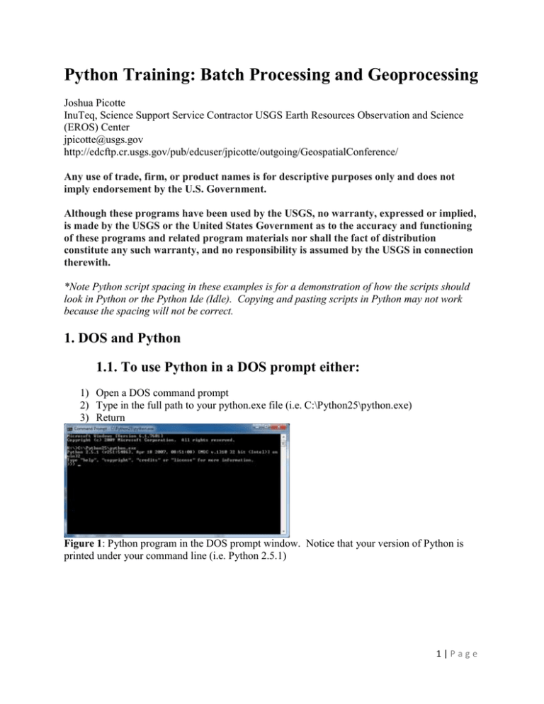
1) Open a DOS command prompt
2) Type in the full path to your python.exe file (i.e. C:\Python25\python.exe)
3) Return
Figure 1: Python program in the DOS prompt window. Notice that your version of Python is
printed under your command line (i.e. Python 2.5.1)
1|Page
1.2. Or, set environmental variable “Path” to the python.exe:
1)
2)
3)
4)
5)
6)
Go to “Control Panel\All Control Panel Items\System” on your computer
Select Advanced system settings
Select Environmental Variables
Highlight “Path” under “System Variables”
Select “Edit”
In the “Variable value:” box type “;” (a semicolon) after the last item in the list of
variables (e.g. E:\Perl\bin) and type in the folder location in that holds your python.exe
file (e.g. E:\Perl\bin; C:\Python25) and click “OK”. Do not put a “;” (a semicolon) after
the Python folder.
-If you set your Python path correctly, you should now be able to access Python using a DOS
prompt.
-To test whether you can use Python in Dos:
1) Open a DOS command prompt
2) Type in: python
3) Return
-You should now be able to type in your python commands (see Figure 1).
2. Python Versions
-You can install multiple versions of Python on your computer; however, you will need to
determine which version you are currently running as the default.
2.1. Determine Current Version of Python
# Print the current version of Python you are using
import sys
print sys.version
2.2. Change Your Computer’s Default Version of Python
-If you have different versions of Python installed, to change the version of Python that your
machine is currently using as the default:
1) Open a DOS command prompt
2) Type in: ftype Python.File=”C:\Python25\python.exe” “%1” %*
(In this example I typed the location of my Python 2.5 python.exe file, you can change
the file location to whichever version of python you want to use.)
3) Return
4) Type in: Assoc .py = Python.File
5) Return
2|Page
3. Multiple File Loops
3.1 os.walk
import os
# Path to input file
InFile = "D:\\Temp\\"
# Walk through nested files in your directory structure.
for root, dirs, files in os.walk(InFile, topdown=False):
for r_in in files:
if r_in.endswith('.tif'):
# Join the path and file together
InRaster = os.path.join(root, r_in)
else:
pass
3.2. Glob
# Examine folders for all files
import glob
# Change * to *.tif if looking for TIF files
InFile = "D:\\Temp\\*"
#Examine each file in the list created by the glob command
for f in glob.glob(InFile):
print f
4.0 Determine Whether File Exists
import os
InFile = "D:\\Temp\\"
# Determine if Path exists, if not, make a directory.
if not os.path.exists(InFile):
# If file doesn’t exist, insert function here…
os.mkdir(InFile)
else:
pass
3|Page
5. ArcGIS
5.1. ArcGIS Versioning
-Determine which version of ArcGIS is installed on your computer:
import _winreg
# Use winreg to check your registry for the version of ArcGIS installed on your machine.
hkey = _winreg.OpenKey(_winreg.HKEY_LOCAL_MACHINE, "SOFTWARE\ESRI\ArcGIS", 0,
_winreg.KEY_READ)
val,typ = _winreg.QueryValueEx(hkey, "RealVersion")
_winreg.CloseKey(hkey)
version = val[0:3]
print version
5.2. ArcGIS 9.*
-Version 9.* uses Python 2.5
# Calling ArcGIS 9.* from Python
import arcgisscripting
gp = arcgisscripting.create()
# gp is the geoprocessing object (i.e. gp.describe()) for calling the different processing functions
# within ArcGIS.
-ArcGIS often requires that you set your workspace folder.
ArcGIS 9.*
# There are multiple ways to tell Arc which folder is your working directory
gp.workspace = “D:/Temp/”
gp.workspace = “D:\\Temp\\”
gp.workspace = r’D:\Temp’
4|Page
5.2. ArcGIS 10.*
ArcGIS Version 10.0 uses Python 2.6 and Version 10.1 uses Python 2.7
# Calling ArcGIS 10.* from Python
import arcpy
# arcpy is the object (i.e. arcpy.Describe()) for calling the different processing functions within
# ArcGIs.
ArcGIS often requires that you set your workspace folder.
ArcGIS 10.*
# Arc 10 requires that you important the environmental module (env)
from arcpy import env
# There are multiple ways to tell Arc which folder is your working directory
env.workspace =“D:/Temp/”
env.workspace = “D:\\Temp\\”
env.workspace = r’D:\Temp’
6. ERDAS Imagine
6.1. Image Command Tool
-Need to create three files:
1) .bat-“Batch” file: Runs the file from DOS
2) .bcf-“Batch Command File”: Contains the ERDAS commands
3) .bls-empty file that ERDAS utilizes
-Pyramids and Statistics example
import os
import shutil
# Change these paths according to your computer setup
InFolder = 'D:\\update_2010\\Review\\'
# Path on your computer to modeler.exe
ERDAS = 'C:\\ERDAS\\Geospatial Imaging 9.3\\bin\\ntx86\\batchprocess.exe'
# BLS-Empty file required by ERDAS
bls_filename = InFolder + 'pystats.bls'
bls = open(bls_filename, 'w')
bls.close()
# BCF-Insert ERDAS command lines here.
bcf_filename = InFolder + 'pystats.bcf'
bcf = open(bcf_filename, 'w')
5|Page
BcfOut = []
for root, dirs, files in os.walk(InFolder, topdown=False):
for img in files:
if img.endswith('.img'):
ImgIn = (os.path.join(root, img)).replace('\\', '/')
Rrd = img.replace('.img', '.rrd')
# Determine whether .rrd images exist
if not os.path.exists(Rrd):
# Insert the image command tool build pyramids here with your file information.
BcfOut.append('imagecommand ' + ImgIn + ' -stats 0 0.0000000000000000e+000 1'\
' 1 Default 256 -aoi none -pyramid 3X3 1 -meter imagecommand' +\
'\n')
else:
pass
else:
pass
bcf.writelines(BcfOut)
bcf.close()
# BAT-Create Bat file to run required ERDAS files
bat_filename = InFolder + 'pystats.bat'
bat = open(bat_filename, 'w')
Lines = '"' + ERDAS + '" -bcffile ' + '"' + bcf_filename.replace('/', '\\') + '" -blsfile "' +\
bls_filename.replace('/', '\\') + '"' + '\n'
bat.writelines(Lines)
bat.close()
# Runs script using DOS. ERDAS Version 9 and below require ERDAS to be open
os.system(bat_filename)
6.2. Modeler .mdls
-Need to create:
1) .bat file
2) .mdl file
-Mdl example
import os
import sys
# sys.argv allows you to enter in extra data in the
# DOS command prompt (i.e. script.py 1739)
PR = sys.argv[1]
6|Page
P = PR[0:2]
R = PR[2:4]
InFolder = 'E:\\BAE\\' +\
'p0' +\
P +\
'r0' +\
R +\
'\\'
Bnb8Folder = InFolder + 'bnb8\\'
BnblcFolder = InFolder + 'bnblc\\'
NlcdFile = 'D:\\ROSES\\NLCD_2006\\' + 'p' + P + 'r' + R + '_nlcd_2006.img'
# Path on your computer to modeler.exe'
ERDAS = 'C:\\ERDAS\\ERDAS Desktop 2011\\bin\\Win32Release\\modeler.exe'
if not os.path.exists(BnblcFolder):
os.mkdir(BnblcFolder)
else:
pass
for root, dirs, files in os.walk(Bnb8Folder, topdown=False):
for raster in files:
if raster.endswith('_bnb8.tif'):
InRaster = Bnb8Folder + raster
OutRaster = BnblcFolder + raster.replace('_bnb8.tif', '_bnblc.tif')
if not os.path.exists(OutRaster):
print '\n\nCreating ' + raster.replace('_bnb8.tif', '_bnblc.tif') + '...'
# BAT
BatName = OutRaster.replace('.tif', '.bat')
MdlName = OutRaster.replace('.tif', '.mdl')
Bat = open(BatName, 'w')
# Write your bat command here. This is the same command your would run in DOS
Bat.writelines('"' + ERDAS + '" ' +\
'"' + MdlName + '"')
Bat.close()
7|Page
# Mdl You can write out any command in ERDAS to a txt file. To find out your commands,
# examine a mdl file that can be saved after your complete your gmd file
Mdl = open(MdlName, 'w')
Mdl.write('SET CELLSIZE MIN;' + '\n' +\
'SET WINDOW Intersection;' + '\n' +\
'SET AOI NONE;' + '\n\n' +\
'Integer RASTER n1_nlcd FILE OLD PUBINPUT NEAREST NEIGHBOR '\
'AOI NONE "' + NlcdFile.replace('\\', '/') + '";\n' +\
'Integer RASTER n2_in FILE OLD PUBINPUT NEAREST NEIGHBOR '\
'AOI NONE "' + InRaster.replace('\\', '/') + '";\n' +\
'Integer RASTER n3_out FILE NEW PUBOUT USEALL THEMATIC BIN '\
'DIRECT DEFAULT 1 BIT UNSIGNED INTEGER "' +\
OutRaster.replace('\\', '/') + '";\n\n' +\
'SET PROJECTION USING n1_nlcd;' + '\n\n' +\
'n3_out = CONDITIONAL {' + '\n' +\
'(($n1_nlcd != 0 && $n1_nlcd != 11 && $n1_nlcd != 21 &&' + '\n' +\
'$n1_nlcd != 22 && $n1_nlcd != 23 && $n1_nlcd != 24 &&' + '\n' +\
'$n1_nlcd != 81 && $n1_nlcd != 82) && ($n2_in >= 95)) 1' + '\n' +\
'};' + '\n' +\
'QUIT;' + '\n'
)
Mdl.close()
# Run Mdl
print '\n\nRunning ' + BatName + '...'
os.system(BatName)
else:
print '\n\n' + raster.replace('_bnb8', '_bnblc') + ' already exists...'
7. GDAL
-Installation directions
Python 2.5
http://www.gis.usu.edu/~chrisg/python/2009/docs/gdal_win.pdf
Python 2.6+
http://pythongisandstuff.wordpress.com/2011/07/07/installing-gdal-and-ogr-for-python-onwindows/
-Or download QGIS to get Python, Gdal, and other open source geospatial packages
https://www.qgis.org/en/site/forusers/download.html
8|Page
7.1. Reading in imagery
import os
from osgeo import gdal
dNBRFile = 'C:\\Temp\\dNBR_test.tif'
# Open Raster image
DT = gdal.Open(dNBRFile)
# Initiate the GeoTransform method
geotransform = DT.GetGeoTransform()
# Number of rows
DTrows = DT.RasterYSize
# Number of columns
DTcols = DT.RasterXSize
# Number of bands
DTbands = DT.RasterCount
# Center of pixel: +15 to move right from the left hand corner of a 30m image
DTX = geotransform[0] + 15
# Center of pixel: -15 to move down 15 meters from the left hand corner of a 30m image
DTY = geotransform[3] -15
# Set the band you want to see
DTband1 = DT.GetRasterBand(1)
# Gdal allows you to read in data as an array.
# The Python module Numpy can allow you to perform more complicated array functions.
DTData = DTband1.ReadAsArray(0,0,DTcols,DTrows)
# (start, stop, step)
for x in range(0, DTrows):
for y in range(0, DTcols):
# Get the X Locations
DTXout = DTX - (30 * x)
# GET the Y Locations
DTYout = DTY + (30 * y)
DTData[x,y]#Extract pixel value
9|Page
8.0 R
8.1. Installation
8.1.1. Install R
-Check to see which version of R is currently compatible with your version of Python (see
http://rpy.sourceforge.net/rpy2/doc-2.4/html/overview.html#installation for details).
-You can download different versions of R from http://cran.r-project.org/bin/windows/base/old/
-Double click the R install-package .exe file to install R on your system.
-Accept all of the R install-package predetermined variables.
8.1.2. Install R Pages
-Open the R program.
- The easiest way to install R packages is to type the command line in R. Download the “rgdal”
and “sp” R packages. Both of these packages will help with performing geospatial calculations
and getting shapefiles and raster files into R. After you type in the package install command for
“rgdal” and “sp” (see below) “hit” the Return button. You will then be prompted to select a
Cran Mirror site for the download. Select a Cran Mirror site.
>install.packages("rgdal", dep=TRUE)
8.1.3. Set System Variables
-Go to: Advance and System Settings; Environmental variables
-Select: Path; Edit; Add “;” and the path to your R.exe file (e.g. ;C:\Program Files\R\R3.1.1\bin) after the last item in the list; Ok
-Add R_HOME as a System variable: New; Variable Name: R_HOME, Variable Value: Path to
R folder (e.g. C:\Program Files\R\R-3.1.1); Ok; Ok
8.1.4. Fix potential robject.py error
-Navigate to your Python \Lib\site-packages\rpy2\robjects folder (e.g.
C:\Python27\ArcGIS10.2\Lib\site-packages\rpy2\robjects).
-Open robject.py in IDLE
-On line 41: Hit return after “tmpf.close()”
-Now, on line 42: type self.__close(tmp)
-Save and close robject.py
-See https://bitbucket.org/lgautier/rpy2/issue/191/unable-to-unlink-file for more details.
10 | P a g e
8.1.5. Install Python Modules
-Install the “pywin32-219.win32-py2.7.exe” python module. The Rpy2 program is dependent on
some information contained within this module. This module must be installed after R.
-Install the “rpy2‑2.4.3.win32‑py2.7.exe” Rpy2 python module (see
http://rpy.sourceforge.net/rpy2/doc-2.4/html/overview.html#download for more details). Accept
all of the program’s suggestions. The RPY2 module will allow Python to communicate with R.
This module must be installed after pywin32 and R.
8.2 Running scripts
-Open Python
import rpy2.robjects as robjects
# Call robjects (Rpy2) to send R commands through R
r = robjects.r
# Calculate the sum of x1 (10) and x2 (40) in Python using R
r('x1=10')
r('x2=40')
VAR1=r('x1+x2')
print VAR1[0]
9.0 DOS
-Use DOS to run .exe’s from command line
9.1. 7zip example
-Assumes path to 7zip (7z) is in your Environments/Paths
import os
# Change the working folder
os.chdir('C:\Users\jpicotte\Desktop\Temp')
# Extract files command
cmd = "7z e L5045028_02820110909_nbr.img.gz"
# Run the command in DOS
os.system(cmd)
11 | P a g e
9.2. Gdal command line example
-Assumes path to gdal\bin is in your Environments/Paths
import os
# Shape to Kml command
cmd = 'ogr2ogr -f "ESRI Shapefile" E:\ROSES\HMS_annual\HmsKml\2004\1028\test.shp'\
'E:\ROSES\HMS_annual\HmsKml\2004\1028\LE70100282004140EDC02_hms.kml'
# Run the command
os.system(cmd)
10.0. Databases
10.1. Sql alchemy
-Use to connect to a database including Mysql, Postgresql, ect.
-Some Databases may require additional python modules to connect properly (i.e. Postgresql
needs psycopg).
from sqlalchemy import *
# Create database engine
Engine=create_engine('mysql://root:password@localhost/database? '\
'charset=utf8&use_unicode=0', pool_recycle=3600)
# Need metadata to create new tables and connect to database
metadata = MetaData(bind=engine)
# Can use this to connect to database
connection = engine.connect()
# Select Query..Prints out all results
# Insert SQL query here…
result = engine.execute("SELECT Id From Param")
# Loop through each row in your results
for row in result:
# Call the row you want to evaluate by its database name
print "Id:", row['Id']
# Make sure to close your query before next query starts
result.close()
12 | P a g e
10.1 Clustering using Scikit (sklearn.cluster)
-Scikit (is a module package that contains many functions for data mining and analysis.
-Clustering based upon X, Y, and Z data can be achieved using sklearn.cluster in the Scikit
module.
-Clustering methods include K-means, Affinity Propagation, Mean-shift, Spectral clustering,
Ward hierarchical clustering, Agglomerative clustering, DBSCAN, and Gaussian mixtures (for
descriptions of each function see http://scikit-learn.org/stable/modules/clustering.html).
-This example focuses on Mean-shift, because you can have many clusters of even size (for a full
explanation see http://scikit-learn.org/stable/modules/clustering.html#mean-shift).
-This example uses Hazard Mapping System fire detection data that is an amalgamation of
GOES, MODIS, and AVHRR fire hot spot detections that can be acquired bi-hourly (see
http://satepsanone.nesdis.noaa.gov/FIRE/fire.html).
-The python Scipy, numpy, and scikit modules need to be installed along with your version of
python.
import csv
import os
import collections
import numpy as np
import pylab as pl
from scipy.spatial import distance
from sklearn.cluster import MeanShift, estimate_bandwidth
InFolder = 'D:\\Workspace\\'
InCsv = InFolder + 'LE70180392012074EDC00_hms.csv'
Hms = ((InCsv.split('\\'))[-1]).replace('.csv', '')
NewCsv = InCsv.replace('.csv', '_group_meanshift_XyOnly.csv')
CluCsv = InCsv.replace('.csv', '_center_meanshift_XyOnly.csv')
NewFig = NewCsv.replace('.csv', '.png')
Onew = open(NewCsv, 'w')
Cnew = open(CluCsv, 'w')
# Pull in data as dictionary using DictReader
Inlabels = ['X', 'Y', 'Date', 'UTC', 'Sensor']
Onew.write('Group,' + ','.join(Inlabels) + '\n')
Cnew.write('Group,TotalPoints,X,Y\n')
13 | P a g e
# Set X axis
# Separate out the coordinates, which is the only data we care about for now
data = csv.DictReader(open(InCsv, 'r').readlines()[1:], Inlabels)
Xcoords = [(float(d['X'])) for d in data if len(d['X']) > 0]
# Set X start, midpoint, and end coordinates for graph outputs
Xsort = np.sort(Xcoords)
XStart = int(Xsort[0] - 5000)
XMid = int(np.mean(Xcoords))
XEnd = int(Xsort[-1]) + 5000
XStartToMid = int((XStart + XMid) / 2)
XMidToEnd = int((XEnd + XMid) / 2)
# Determine the total number of Coordinates
TotalNum = len(Xsort)
del data
# Set Y axis
# Separate out the coordinates, which is the only data we care about for now
data = csv.DictReader(open(InCsv, 'r').readlines()[1:], Inlabels)
Ycoords = [(float(d['Y'])) for d in data if len(d['Y']) > 0]
Ysort = np.sort(Ycoords)
YStart = int(Ysort[0] - 5000)
YMid = int(np.mean(Ycoords))
YEnd = int(Ysort[-1]) + 5000
YStartToMid = int((YStart + YMid) / 2)
YMidToEnd = int((YEnd + YMid) / 2)
del data
# Load data
# Load everything into a Numpy array.
# Make sure to only use the columns (usecols=), in this
# case X and Y that you require. Adding more columns will affect the results
X = np.loadtxt(open(InCsv, "rb"), delimiter=",", skiprows=1, usecols=(0, 1))
# That this function takes time at least quadratic in n_samples. For large datasets,
# it’s wise to set that parameter to a small value.
# quantile : float, default 0.3
# should be between [0, 1] 0.5 means that the median of all pairwise
# distances is used.
bandwidth = estimate_bandwidth(X, quantile=0.01, n_samples=len(X))
14 | P a g e
# bandwidth : float, optional
# Bandwidth used in the RBF kernel.
# If not given, the bandwidth is estimated using sklearn.cluster.estimate_bandwidth;
# see the documentation for that function for hints on scalability.
ms = MeanShift(bandwidth=bandwidth, bin_seeding=True)
ms.fit(X)
labels = ms.labels_
cluster_centers = ms.cluster_centers_
labels_unique = np.unique(labels)
n_clusters_ = len(labels_unique)
pl.figure(1)
pl.clf()
# Determine the number of points in each cluster
counter = collections.Counter(labels)
# Use Pylabs unique set of color combinations (in this case Set1) to
# create unique colors for each Mean Shift cluster
colors = pl.cm.Set1(np.linspace(0, 1, len(labels_unique)))
DataOut = []
for k, col in zip(range(n_clusters_), colors):
my_members = labels == k
cluster_center = cluster_centers[k]
# Write out cluster center points
ClusX = cluster_center[0]
ClusY = cluster_center[1]
# Keeps track of how many points make up each cluster
Count = counter[k]
ClusOut = (str(k) + ',' +
str(Count) + ',' +
str(ClusX) + ',' +
str(ClusY) + '\n')
Cnew.write(ClusOut)
15 | P a g e
# markersize is scaled by twice the number of the count
pl.plot(cluster_center[0], cluster_center[1], 'o', markerfacecolor=col,
markeredgecolor='k', markersize=int(Count * 2))
pl.plot(X[my_members, 0], X[my_members, 1], 'o', markerfacecolor=col,
markeredgecolor='k', markersize=3)
pl.xticks([XStart, XStartToMid, XMid, XMidToEnd, XEnd])
pl.yticks([YStart, YStartToMid, YMid, YMidToEnd, YEnd])
for i in X[my_members]:
# join lines together
InLine = str(k) + ',' + ','.join(str(x)
for x in i) + ','
# Need to convert float Date/time to strings
LineOut = InLine.replace(
'.0,',
',')
Lo = LineOut.split(',')
x = Lo[1]
y = Lo[2]
data = csv.DictReader(open(InCsv, 'r').readlines()[1:], Inlabels)
for d in data:
if y == d['Y'] and x == d['X']:
Date = d['Date']
Utc = d['UTC']
Sensor = d['Sensor']
Out = LineOut +\
Date + ',' +\
Utc + ',' +\
Sensor + '\n'
DataOut.append(Out)
else:
pass
pl.title(
Hms +
'\nTotal Number of Detections: %d' %
TotalNum +
'\nTotal Number of Clusters: %d' %
n_clusters_,
fontweight="bold",
fontsize=10)
# Saves the figure
pl.savefig(NewFig)
16 | P a g e
Onew.writelines(set(DataOut))
Onew.close()
Cnew.close()
Figure 2: Example output from clustering algorithm. Notice that grouped points are on top of
the cluster centers, and that the clusters and centers have the same color. Plot centers have also
been scaled in size to have an area that is equal to twice the number of points.
17 | P a g e