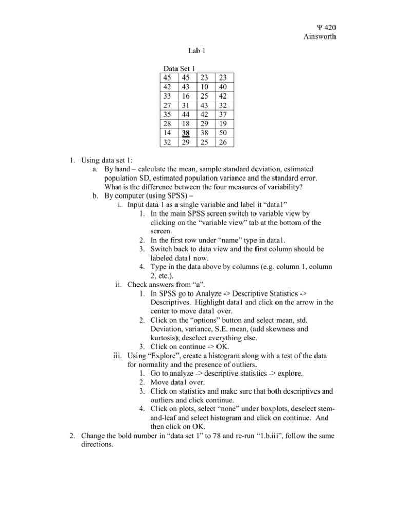
Ψ 420
Ainsworth
Lab 1
Data Set 1
45 45
42 43
33 16
27 31
35 44
28 18
14 38
32 29
23
10
25
43
42
29
38
25
23
40
42
32
37
19
50
26
1. Using data set 1:
a. By hand – calculate the mean, sample standard deviation, estimated
population SD, estimated population variance and the standard error.
What is the difference between the four measures of variability?
b. By computer (using SPSS) –
i. Input data 1 as a single variable and label it “data1”
1. In the main SPSS screen switch to variable view by
clicking on the “variable view” tab at the bottom of the
screen.
2. In the first row under “name” type in data1.
3. Switch back to data view and the first column should be
labeled data1 now.
4. Type in the data above by columns (e.g. column 1, column
2, etc.).
ii. Check answers from “a”.
1. In SPSS go to Analyze -> Descriptive Statistics ->
Descriptives. Highlight data1 and click on the arrow in the
center to move data1 over.
2. Click on the “options” button and select mean, std.
Deviation, variance, S.E. mean, (add skewness and
kurtosis); deselect everything else.
3. Click on continue -> OK.
iii. Using “Explore”, create a histogram along with a test of the data
for normality and the presence of outliers.
1. Go to analyze -> descriptive statistics -> explore.
2. Move data1 over.
3. Click on statistics and make sure that both descriptives and
outliers and click continue.
4. Click on plots, select “none” under boxplots, deselect stemand-leaf and select histogram and click on continue. And
then click on OK.
2. Change the bold number in “data set 1” to 78 and re-run “1.b.iii”, follow the same
directions.
Ψ 420
Ainsworth
Data Set 2
Treatment Group
Control Group
Response
Yes
No
34
19
26
27
60
46
53
53
106
3. Using data set 2:
a. By hand – calculate the chi-square for the relationship between the two
discrete variables. Is there a relationship? Refer to table A.2 in the
appendix.
b. By computer – check your answer to “a”.
i. Using the same SPSS data window, create a new variable and label
it “Group” -> click on values and 1 = treatment and 2 = control.
Create a new variable and label it “Response” -> click on values
and 1 = yes and 2 = no.
ii. In the group variable enter 53 “1’s” down the column and then
enter 53 “2’s” down the column.
iii. In the Response column enter 34 “1’s” and then 19 “2’s”; enter 26
“1’s” and then 27 “2’s”.
iv. Go to analyze -> descriptive statistics -> crosstabs. Put group in
rows and response in columns. Click on statistics and select chisquare, click on continue -> OK.
Ψ 420
Ainsworth
Data Set 3
Height of Number of
Plant
Plant
Seeds
1
20
42
2
17
38
3
19
45
4
21
48
5
20
44
6
20
43
7
22
46
8
21
45
9
16
39
10
24
55
11
22
49
12
24
55
13
21
43
14
19
38
15
21
51
16
20
46
17
15
40
4. Using data set 3:
a. By hand – compute correlation and regression
for the two continuous variables.
b. By computer – check the answers from “a”
and annotate the output.
i. Create two new variables “height” and
“number”. Enter the data the way it is
seen to the left (without the plant
numbers)
ii. Analyze -> Correlate -> Bivariate.
Highlight both height and number and
move them over to the variables box.
Click on OK.
iii. Analyze -> Regression -> Linear.
Move number over into “dependent”
and height over into “independent(s)”.
Click on OK.
c. Generate a scatterplot and describe it.
i. Graphs -> Legacy Dialogs ->
“Scatter/dot…”. Click on simple ->
Define.
Move height into x-axis and
number into y-axis. Click on OK.
Data set 3
Group
Anger Level
1
Control
15
2
Control
12
3
Control
12
4
Control
5
5
Control
11
6
Control
13
7
Control
9
8
Control
7
9
Control
10
10 Control
7
11 Treatment
8
12 Treatment
10
13 Treatment
6
14 Treatment
5
15 Treatment
7
16 Treatment
5
17 Treatment
9
18 Treatment
8
19 Treatment
3
20 Treatment
4
5. Using data set 3:
a. By hand –
i. Perform an independent samples ttest.
ii. Perform a dependent samples t-test
(assuming each person is in both the
treatment and control, the answers #1
and #11 are from the same person,
etc.)
b. By computer –
i. Redo “a” as an independent samples ttest to check “a” answer. Annotate
the output.
1. Create a group and an anger
variable, label the group
variable appropriately.
2. Analyze – Compare Means –
Independent samples T-Test.
Move Anger into test variable
and group into grouping
variable -> Define groups and
put a 1 in group1 and a 2 in
Ψ 420
Ainsworth
group 2. Continue -> OK.
ii. Perform a matched pair (dependent samples) t-test. Assume that
every subject participates in the treatment and control. Annotate
the output.
1. Create two new variables; control and treatment.
2. Rearrange the data to the in data set 3 so that the first
person has a score of 15 on a control and a score of 8 on
treatment, and so on down the .
3. Analyze -> Compare Means -> Paired samples T-Test.
Highlight both treatment and control -> move them both
over to create a pair of variables in the “paired variables”
box. Click on OK.
iii. How are “i” and “ii” different and why?