STA 6207 – Exam 1 – Fall 2014
PRINT Name _____________________
Conduct all tests at the  = 0.05 Significance level.
All Models on test are of the forms:
Scalar: Y   0  1 X 1  ...   p X p  
 ~ N  0,  2  independent Matrix: Y  Xβ  ε ε ~ N  0,  2I 
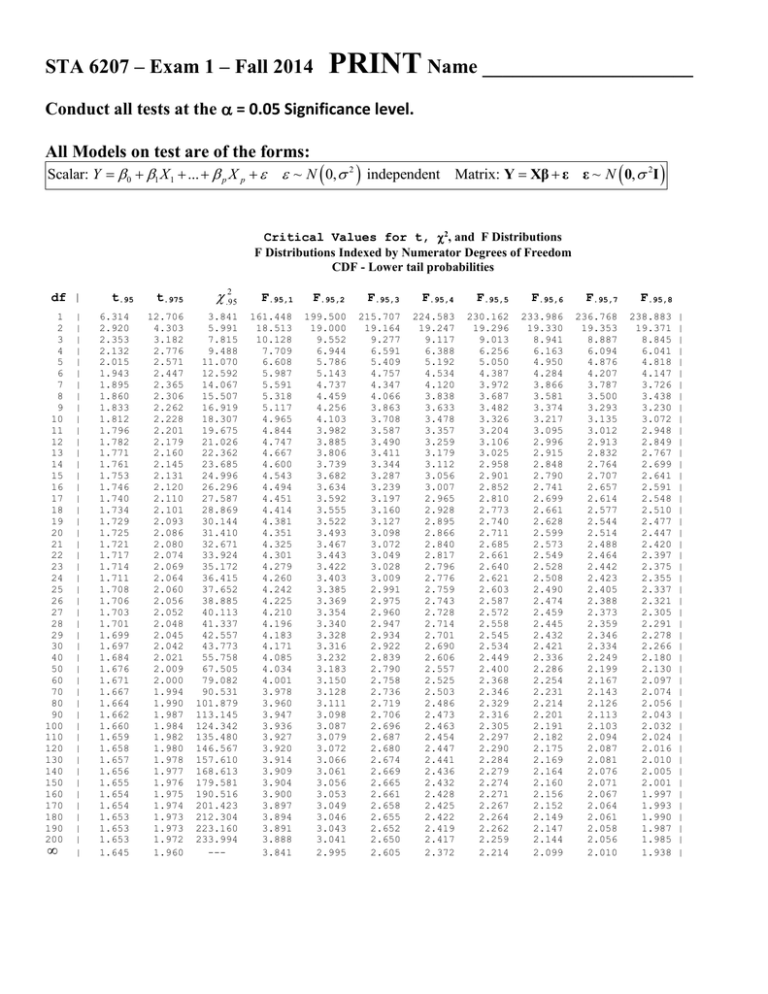
Critical Values for t, 2, and F Distributions
F Distributions Indexed by Numerator Degrees of Freedom
CDF - Lower tail probabilities
df |
1
2
3
4
5
6
7
8
9
10
11
12
13
14
15
16
17
18
19
20
21
22
23
24
25
26
27
28
29
30
40
50
60
70
80
90
100
110
120
130
140
150
160
170
180
190
200

|
|
|
|
|
|
|
|
|
|
|
|
|
|
|
|
|
|
|
|
|
|
|
|
|
|
|
|
|
|
|
|
|
|
|
|
|
|
|
|
|
|
|
|
|
|
|
|
t.95
6.314
2.920
2.353
2.132
2.015
1.943
1.895
1.860
1.833
1.812
1.796
1.782
1.771
1.761
1.753
1.746
1.740
1.734
1.729
1.725
1.721
1.717
1.714
1.711
1.708
1.706
1.703
1.701
1.699
1.697
1.684
1.676
1.671
1.667
1.664
1.662
1.660
1.659
1.658
1.657
1.656
1.655
1.654
1.654
1.653
1.653
1.653
1.645
t.975
 .295
F.95,1
F.95,2
F.95,3
F.95,4
F.95,5
F.95,6
F.95,7
F.95,8
12.706
4.303
3.182
2.776
2.571
2.447
2.365
2.306
2.262
2.228
2.201
2.179
2.160
2.145
2.131
2.120
2.110
2.101
2.093
2.086
2.080
2.074
2.069
2.064
2.060
2.056
2.052
2.048
2.045
2.042
2.021
2.009
2.000
1.994
1.990
1.987
1.984
1.982
1.980
1.978
1.977
1.976
1.975
1.974
1.973
1.973
1.972
1.960
3.841
5.991
7.815
9.488
11.070
12.592
14.067
15.507
16.919
18.307
19.675
21.026
22.362
23.685
24.996
26.296
27.587
28.869
30.144
31.410
32.671
33.924
35.172
36.415
37.652
38.885
40.113
41.337
42.557
43.773
55.758
67.505
79.082
90.531
101.879
113.145
124.342
135.480
146.567
157.610
168.613
179.581
190.516
201.423
212.304
223.160
233.994
---
161.448
18.513
10.128
7.709
6.608
5.987
5.591
5.318
5.117
4.965
4.844
4.747
4.667
4.600
4.543
4.494
4.451
4.414
4.381
4.351
4.325
4.301
4.279
4.260
4.242
4.225
4.210
4.196
4.183
4.171
4.085
4.034
4.001
3.978
3.960
3.947
3.936
3.927
3.920
3.914
3.909
3.904
3.900
3.897
3.894
3.891
3.888
3.841
199.500
19.000
9.552
6.944
5.786
5.143
4.737
4.459
4.256
4.103
3.982
3.885
3.806
3.739
3.682
3.634
3.592
3.555
3.522
3.493
3.467
3.443
3.422
3.403
3.385
3.369
3.354
3.340
3.328
3.316
3.232
3.183
3.150
3.128
3.111
3.098
3.087
3.079
3.072
3.066
3.061
3.056
3.053
3.049
3.046
3.043
3.041
2.995
215.707
19.164
9.277
6.591
5.409
4.757
4.347
4.066
3.863
3.708
3.587
3.490
3.411
3.344
3.287
3.239
3.197
3.160
3.127
3.098
3.072
3.049
3.028
3.009
2.991
2.975
2.960
2.947
2.934
2.922
2.839
2.790
2.758
2.736
2.719
2.706
2.696
2.687
2.680
2.674
2.669
2.665
2.661
2.658
2.655
2.652
2.650
2.605
224.583
19.247
9.117
6.388
5.192
4.534
4.120
3.838
3.633
3.478
3.357
3.259
3.179
3.112
3.056
3.007
2.965
2.928
2.895
2.866
2.840
2.817
2.796
2.776
2.759
2.743
2.728
2.714
2.701
2.690
2.606
2.557
2.525
2.503
2.486
2.473
2.463
2.454
2.447
2.441
2.436
2.432
2.428
2.425
2.422
2.419
2.417
2.372
230.162
19.296
9.013
6.256
5.050
4.387
3.972
3.687
3.482
3.326
3.204
3.106
3.025
2.958
2.901
2.852
2.810
2.773
2.740
2.711
2.685
2.661
2.640
2.621
2.603
2.587
2.572
2.558
2.545
2.534
2.449
2.400
2.368
2.346
2.329
2.316
2.305
2.297
2.290
2.284
2.279
2.274
2.271
2.267
2.264
2.262
2.259
2.214
233.986
19.330
8.941
6.163
4.950
4.284
3.866
3.581
3.374
3.217
3.095
2.996
2.915
2.848
2.790
2.741
2.699
2.661
2.628
2.599
2.573
2.549
2.528
2.508
2.490
2.474
2.459
2.445
2.432
2.421
2.336
2.286
2.254
2.231
2.214
2.201
2.191
2.182
2.175
2.169
2.164
2.160
2.156
2.152
2.149
2.147
2.144
2.099
236.768
19.353
8.887
6.094
4.876
4.207
3.787
3.500
3.293
3.135
3.012
2.913
2.832
2.764
2.707
2.657
2.614
2.577
2.544
2.514
2.488
2.464
2.442
2.423
2.405
2.388
2.373
2.359
2.346
2.334
2.249
2.199
2.167
2.143
2.126
2.113
2.103
2.094
2.087
2.081
2.076
2.071
2.067
2.064
2.061
2.058
2.056
2.010
238.883
19.371
8.845
6.041
4.818
4.147
3.726
3.438
3.230
3.072
2.948
2.849
2.767
2.699
2.641
2.591
2.548
2.510
2.477
2.447
2.420
2.397
2.375
2.355
2.337
2.321
2.305
2.291
2.278
2.266
2.180
2.130
2.097
2.074
2.056
2.043
2.032
2.024
2.016
2.010
2.005
2.001
1.997
1.993
1.990
1.987
1.985
1.938
|
|
|
|
|
|
|
|
|
|
|
|
|
|
|
|
|
|
|
|
|
|
|
|
|
|
|
|
|
|
|
|
|
|
|
|
|
|
|
|
|
|
|
|
|
|
|
|
Q.1. Regression models were fit, relating height (Y, in mm) to hand length (X1, in mm), foot length (X2, in mm)
and gender (X3=1 if male, 0 if female) based on a sample of 80 males and 75 females. Consider these 4 models:
Model 1: E Y    0  1 X 1   2 X 2  3 X 3  13 X 1 X 3   23 X 2 X 3
Model 2: E Y    0  1 X 1   2 X 2  3 X 3
Model 3 (Males Only): E Y    0  1 X 1   2 X 2
Model 4 (Females Only): E Y    0   1 X 1   2 X 2
ANOVA
Regression
Residual
Total
Intercept
Hand
Foot
Male
MaleHand
MaleFoot
Model1
df
5
149
154
ANOVA
SS
1201091
157138
1358229
Coefficients
Standard Error
744.14
83.68
2.38
0.51
1.73
0.39
-304.72
125.47
0.91
0.68
0.65
0.52
Regression
Residual
Total
Intercept
Hand
Foot
Male
Model2
df
3
151
154
ANOVA
SS
1193101
165128
1358229
CoefficientsStandard Error
582.16
60.55
2.81
0.34
2.06
0.26
39.61
8.50
Regression
Residual
Total
Intercept
Hand
Foot
Model3
df
ANOVA
2
77
79
SS
208298
88305
296603
Coefficients
Standard Error
439.42
97.49
3.29
0.47
2.38
0.35
Regression
Residual
Total
Intercept
Hand
Foot
Model4
df
2
72
74
SS
110552
68833
179385
Coefficients
Standard Error
744.14
79.67
2.38
0.49
1.73
0.37
p.1.a. Confirm the equivalence of the regression coefficients (but not standard errors) based on the appropriate
models (Hint: set up the fitted equations based on the two models):
Females:
Males:
p.1.b. Test H0: = 0 (No interactions between Hand and Gender or Foot and Gender).
Test Statistic: __________________ Rejection Region: ______________________ p-value > or < 0.05?
p.1.c. Use Hartley’s Test to test whether the error variances among the individual regressions are equal:
t
1

B   ln  MSE    i ln  si2  
C
i 1

1  t 1
1 
C  1



i

3  t  1  i 1

Test Statistic B = _____________________ Rejection Region: ________________ p-value > or < 0.05?
p.1.d. What fraction of the total variation in height is explained by the set of predictors: hand length, foot length,
and gender (but no interactions)?
p.1.e. Compute the standard deviations among the 80 Male heights and among the 75 Female heights (ignoring
hand and foot length).
Males: SD = ___________________________
Females: SD = _________________________________
Q.2. A study related Personal Best Shot Put distance (Y, in meters) to best preseason power clean lift (X, in
kilograms). The following models were fit, based on a sample of n = 24 male collegiate shot putters:
^
Model 1: E Y   0  1 X
SSE1  43.41
R12  .686
Y  X   4.4353  0.0898 X
Model 2: E Y   0  1 X   2 X 2
SSE2  37.41
R22  .729
Y X , X 2  12.08  0.3285 X  0.00084 X 2
^


p.2.a. Use Model 2 to test H0: (Y is not related to X)





Test Statistic____________________ Rejection Region: ____________________
Reject H0? Yes
or No
Reject H0? Yes
or No
p.2.b. Use Models 1 and 2 to test H0: (Y is linearly related to X)







Test Statistic: ___________________ Rejection Region: ____________________
p.2.c. Give an estimate of the level of X is that maximizes E{Y}.
X* = ___________________________
Q.3. A study was conducted to determine whether having been exposed to an advertisement claiming a natural
ingredient is contained in a perfume had an effect on subjects’ rating of the perfume’s scent. There were 112
subjects of which, 56 were exposed to the ad, and 56 were not. We fit the following regression model:
Yi  0  1 X i   i
i  1,...,112
X'X
1 if Subject i was exposed to the ad
Xi  
0 if Subject i was not exposed to the ad
X'Y
112
56
56
56
587
337
Y'Y
3683.05
p.3.a. First, we fit a model with only an intercept term, what will P0  X 0  X 0 ' X 0  X 0 ' be (symbolically, do
1
not write out a 112x112 matrix!)? Compute R(0).
P0 = ______________________________ R(0) = ______________________________
p.3.b. Compute  X'X 
1
^
and β
NOTE: Write  X'X 
1
as
1
A for the appropriate A
X'X
p.3.c. Compute R(0 , 1) , R(0), and MSResidual
R(0 , 1) = ________________ R(0) = _________________ MSResidual = __________________
p.3.d. Use the t-test and the F-test to test H0: 0 vs HA≠

















t-Statistic: ____________________ Rejection Region: ___________________________
F-Statistic: ____________________ Rejection Region: ___________________________
Q.4. An experiment was conducted to measure the subsoil pressure of a steel ground roller. There were 3
replicates at each of 4 depths (X=5, 10, 15, 20 cm). The response was measured force (100s of Newtons).
^
The fitted regression equation is Y  49.371  2.036 X
We want to test H0: E{Yj} = 0 + 1Xj
j
X_j
1
2
3
4
Ybar_j SD_j
5
40.38
10
28.87
15
16.23
20
11.15
HA: E{Yj} = j ≠ 0 + 1Xj
Yhat_j
Pure Error
Lack of Fit
4.32
6.83
3.76
4.48
p.4.a. Compute the Pure Error Sum of Squares and Degrees of Freedom. Hint: What is SD_j equal to?
SSPE = __________________________________ dfPE = _________________________________
p.4.b. Compute the Lack-of-Fit Sum of Squares and Degrees of Freedom.
SSLF = __________________________________ dfLF = _________________________________
p.4.c. Conduct the F-test for Lack-of-Fit
Test Statistic: ________________________ Rejection Region: ______________ Reject H0? Yes / No
Q.5. A series of models were fit, relating Average January High Temperature (Y, in degrees F) to Elevation (X1,
in 100s ft above sea level), and Latitude (degrees North Lat) for n = 369 weather stations in Texas. Latitude
and Elevation were centered in the regression models.
CP 
SS Re s Model
 2 p 'n
MSRes Complete
AIC  n ln SS Re s Model   2 p 'n ln( n)
SBC  BIC  n ln SS Re s Model   ln( n) p 'n ln( n)
Variables in Model
ELEV ( E )
LAT ( L )
E,L
E,L,E*L
E,L,E^2,L^2
E,L,E*L,E^2,L^2
SS(RES) C_p
AIC
SBC
7986.3
4764.2
1138.6
1146.4
1168.0
429.2
437.0
616.2
32.8
195.2
207.0
603.9
26.9
205.4
575.0
10.3
173.7
565.2
6
169.3
192.8
p.5.a. Complete the table.
p.5.b. Based on each criteria, which model do you choose?
Cp: _____________________________ AIC: ____________________
SBC: ______________________