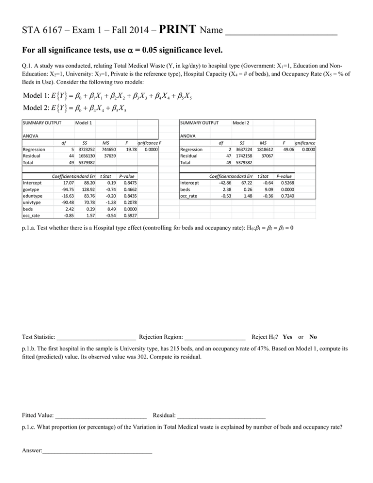
STA 6167 – Exam 1 – Fall 2014 – PRINT Name _______________________
For all significance tests, use  = 0.05 significance level.
Q.1. A study was conducted, relating Total Medical Waste (Y, in kg/day) to hospital type (Government: X 1=1, Education and NonEducation: X2=1, University: X3=1, Private is the reference type), Hospital Capacity (X4 = # of beds), and Occupancy Rate (X5 = % of
Beds in Use). Consider the following two models:
Model 1: E Y    0  1 X 1   2 X 2   3 X 3   4 X 4   5 X 5
Model 2: E Y    0   4 X 4   5 X 5
SUMMARY OUTPUT
Model 1
SUMMARY OUTPUT
ANOVA
ANOVA
df
Regression
Residual
Total
Intercept
govtype
eduntype
univtype
beds
occ_rate
Model 2
SS
5 3723252
44 1656130
49 5379382
MS
744650
37639
F Significance F
19.78
0.0000
Coefficients
Standard Error t Stat
P-value
17.07
88.20
0.19
0.8475
-94.75
128.92
-0.74
0.4662
-16.63
83.76
-0.20
0.8435
-90.48
70.78
-1.28
0.2078
2.42
0.29
8.49
0.0000
-0.85
1.57
-0.54
0.5927
df
Regression
Residual
Total
Intercept
beds
occ_rate
SS
MS
2 3637224 1818612
47 1742158
37067
49 5379382
F Significance F
49.06
0.0000
Coefficients
Standard Error t Stat
P-value
-42.86
67.22
-0.64
0.5268
2.38
0.26
9.09
0.0000
-0.53
1.48
-0.36
0.7240
p.1.a. Test whether there is a Hospital type effect (controlling for beds and occupancy rate): H 0:







Test Statistic: __________________________ Rejection Region: ____________________
Reject H 0? Yes
or
No
p.1.b. The first hospital in the sample is University type, has 215 beds, and an occupancy rate of 47%. Based on Model 1, compute its
fitted (predicted) value. Its observed value was 302. Compute its residual.
Fitted Value: ______________________________
Residual: _____________________________
p.1.c. What proportion (or percentage) of the Variation in Total Medical waste is explained by number of beds and occupancy rate?
Answer:____________________________________
Q.2. A study related Personal Best Shot Put distance (Y, in meters) to best preseason power clean lift (X, in kilograms). The following
models were fit, based on a sample of n = 24 male collegiate shot putters:
^
Model 1: E Y   0  1 X
SSE1  43.41
R12  .686
Y  X   4.4353  0.0898 X
Model 2: E Y   0  1 X   2 X 2
SSE2  37.41
R22  .729
Y X , X 2  12.08  0.3285 X  0.00084 X 2
^


p.2.a. Use Model 2 to test H0: (Y is not related to X)





Test Statistic: __________________________ Rejection Region: ____________________
Reject H0? Yes
or
No
Reject H 0? Yes
or
No
p.2.b. Use Models 1 and 2 to test H0: (Y is linearly related to X)







Test Statistic: __________________________ Rejection Region: ____________________
p.2.c. Obtain the predicted value from each model for a man with best power clean of 175 kg.

Model 1: _____________________________________________ Model 2: __________________________________________
Q.3. A regression model is fit relating weight (Y, in lbs) to height (X, in inches) among n=139 WNBA players (treating this as a
random sample of all female athletes from sports such as basketball and volleyball). The results from the regression, and the residual
versus fitted plot are given below.
ANOVA
df
Regression
Residual
Total
SS
1 45933.13
137 35074.41
138 81007.54
Coefficients
Standard Error
Intercept -212.05
28.78
Height
5.32
0.40
p.3.a. Test H0: 1 = 0 (Weight is not associated with Height) based on the t-test.
Test Statistic: __________________________ Rejection Region: ____________________
Reject H 0? Yes
or
No
Reject H 0? Yes
or
No
p.3.b. Test H0: 1 = 0 (Weight is not associated with Height) based on the F-test.
Test Statistic: __________________________ Rejection Region: ____________________
p.3.c. The residual plot appears to display non-constant error variance. A regression of the squared residuals on height (X) is fit, and
the ANOVA is given below. Conduct the Breusch-Pagan test to test whether the errors are related to X. Do you reject the null
hypothesis of constant variance? Yes or No
ANOVA
df
Regression
Residual
Total
SS
1 1070500
137 44788405
138 45858905
Test Statistic: __________________________ Rejection Region: ____________________
Reject H 0? Yes
or
No
Q.4. An experiment was conducted as a Completely Randomized Design (1-Way ANOVA) to compare t = 4 methods of packaging
steaks, in terms of the amount of bacteria measured after 9 days of storage. There were ni = 3 replicates per treatment. The treatment
means and sums of squares were:
Y 1  7.48 Y 2  5.50 Y 3  7.26 Y 4  3.36
4

 ni Y i  Y 
i 1

2
 32.87
4
  n  1 s
i 1
i
2
i
 0.93 
p.4.a. Conduct the F-test for testing H0: 
Test Statistic: __________________________ Rejection Region: ____________________
Reject H 0? Yes
or
No
p.4.b. Compute Tukey’s Honest Significant Difference for simultaneously comparing all pairs of packages, with a family-wise error
rate of 0.05. Identify significant differences among all pairs of means.
Trt4
Trt2
Trt3
Trt1
p.4.c. Compute Bonferroni’s Minimum Significant Difference for simultaneously comparing all pairs of packages, with a family-wise
error rate of 0.05
Trt4
Trt2
Trt3
Trt1
Q.5 A data set consisted of n = 32 observations on the variables Y, X1, X2, X3, and X4. Error Sum of Squares = SSE for each of all
possible models. For each model, the variables that are in the model are also shown. Use this information to answer the
questions following the table. The Total Sum of Squares = SSTO = 1150.
#Variables
SSE
1
1
1
1
2
2
2
2
2
2
3
3
3
3
4
Cp
330
448
505
785
255
284
290
295
402
445
245
253
255
290
243
AIC
SBC=BIC
#N/A
#N/A
#N/A
#N/A
#N/A
#N/A
#N/A
#N/A
#N/A
#N/A
#N/A
#N/A
#N/A
#N/A
#N/A
#N/A
#N/A
#N/A
#N/A
#N/A
#N/A
#N/A
#N/A
#N/A
#N/A
#N/A
#N/A
#N/A
#N/A
#N/A
#N/A
#N/A
#N/A
Vars in Model
X2
X3
X1
X4
X2,X4
X2,X3
X1,X3
X1,X2
X1,X4
X3,X4
X1,X2,X4
X1,X2,X3
X2,X3,X4
X1,X3,X4
X1,X2,X3,X4
p.5.a. Complete the table by computing Cp, AIC, and SBC=BIC for the best models with 1,2,3, and 4 independent variables.
p.5.b. Give the best model (in terms of which independent variables to be included), based on each criteria.
Cp: ________________________ AIC: _____________________________ SBC=BIC: _________________________
Q.6. A linear regression model was fit, relating the electric potential (Y) to the current density (X) for a series of n=18 consecutively
observed pairs of X and Y.
Model: Yt   0  1 X t   t
 t ~ N  0, 2 
 t   t 1   t
p.6.a. The estimated regression coefficients and standard errors for ordinary least squares are given below. Obtain a 95% Confidence
Interval for the slope coefficient for current density (1).
Coefficients:
Estimate Std. Error t value Pr(>|t|)
(Intercept) 891.460256
4.290707 207.76
<2e-16 ***
x
-0.431633
0.009523 -45.33
<2e-16 ***
Lower Bound: _________________________________
Upper Bound: _____________________________________
p.6.b. The Durbin-Watson test is used to test H0:  = 0. The test statistic and P-value are given below. Do you conclude that the errors
are serially correlated (not independent)? Yes or No
lag Autocorrelation D-W Statistic p-value
1
0.4923645
0.668015
0
p.6.c. The estimated regression coefficients and standard errors for estimated generalized least squares are given below. Obtain a 95%
Confidence Interval for the slope coefficient for current density (1).
Coefficients:
Value Std.Error
t-value p-value
(Intercept) 895.8873 9.161308 97.79033
0
x
-0.4488 0.018576 -24.16305
0
Lower Bound: _________________________________
Upper Bound: _____________________________________