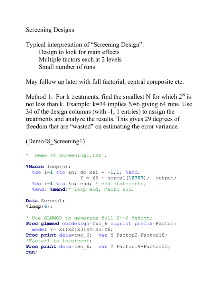
Screening Designs
Typical interpretation of “Screening Design”:
Design to look for main effects
Multiple factors each at 2 levels
Small number of runs
May follow up later with full factorial, central composite etc.
Method 1: For k treatments, find the smallest N for which 2N is
not less than k. Example: k=34 implies N=6 giving 64 runs. Use
34 of the design columns (with -1, 1 entries) to assign the
treatments and analyze the results. This gives 29 degrees of
freedom that are “wasted” on estimating the error variance.
(Demo48_Screening1)
*
Demo 48_Screening1.txt ;
%Macro loop(n);
%do i=1 %to &n; do x&i = -1,1; %end;
Y = X5 + normal(12307);
%do i=1 %to &n; end; * end statements;
%end; %mend;* loop end, macro end;
output;
Data Screen1;
%loop(6);
* Use GLMMOD to generate full 2**6 design;
Proc glmmod outdesign=two_6 noprint prefix=Factor;
model Y= X1|X2|X3|X4|X5|X6;
Proc print data=two_6; var Y Factor2-Factor18;
*Factor1 is intercept;
Proc print data=two_6; var Y Factor19-Factor35;
run;
* Run Main Effects Model;
ods listing close; * turn off output;
ods output ParameterEstimates=Effects;
PROC REG data=two_6;
model Y = Factor2-Factor35;
run; quit;
ods listing;
*data set;
proc print data=Effects; run;
proc print data=Effects; var variable label tValue
Probt;
where probt<0.10/34; *Bonferroni;
run;
Partial output:
O
b
s
Y
F
A
C
T
O
R
2
1
2
3
4
5
6
7
8
0.09060
-1.82867
2.51503
-0.25050
-0.93802
-1.22115
1.43334
-0.99588
-1
-1
-1
-1
-1
-1
-1
-1
61 -1.32861 1
62 -1.23220 1
63 0.42493 1
64 2.04751 1
Obs
1
2
3
F
A
C
T
O
R
3
-1
-1
-1
-1
-1
-1
-1
-1
1
1
1
1
Variable
Intercept
FACTOR2
FACTOR3
F
A
C
T
O
R
4
F
A
C
T
O
R
5
F
A
C
T
O
R
6
1 -1 1
1 -1 1
1 -1 1
1 -1 1
1 -1 1
1 -1 1
1 -1 1
1 -1 1
(53 more
1 1 1
1 1 1
1 1 1
1 1 1
F
A
C
T
O
R
7
F
A
C
T
O
R
8
F
A
C
T
O
R
9
1 -1
1 -1
1 -1
1 -1
1 -1
1 -1
1 -1
1 -1
lines
1 1
1 1
1 1
1 1
-1
-1
-1
-1
1
1
1
1
of
1
1
1
1
DF Estimate
1 -0.00390
1 -0.00559
1 -0.11980
F
A
C
T
O
R
1
0
F
A
C
T
O
R
1
1
F
A
C
T
O
R
1
2
F
A
C
T
O
R
1
3
F
A
C
T
O
R
1
4
F
A
C
T
O
R
1
5
F
A
C
T
O
R
1
6
F
A
C
T
O
R
1
7
F
A
C
T
O
R
1
8
1 1 -1
1 1 -1
1 1 -1
1 1 -1
-1 -1 1
-1 -1 1
-1 -1 1
-1 -1 1
output)
1 1 1
1 1 1
1 1 1
1 1 1
1
1
1
1
-1
-1
-1
-1
-1
-1
-1
-1
1
1
1
1
-1
-1
-1
-1
1
1
1
1
1
1
1
1
-1
-1
-1
-1
-1
-1
1
1
-1
-1
1
1
1
1
-1
-1
1
1
-1
-1
1
1
1
1
1
1
1
1
1
1
1
1
1 -1 -1
1 -1 -1
1 1 1
1 1 1
tValue
-0.03
-0.05
-1.05
Probt
0.9729
0.9611
0.3006
Label
Intercept
x1
x2
(30 more lines)
33 FACTOR33
1 -0.18170 -1.60 0.1207 x6
34 FACTOR34
1
0.35579 3.13 0.0040 x1*x6
35 FACTOR35
1
0.28406 2.50 0.0184 x2*x6
---------------------------------------------------Obs
Variable
Label
tValue
Probt
17
FACTOR17
x5
9.86 <.0001
Method 2 Plackett-Burman Plans:
Must have number of rows n=2 or n= 4m for integer m.
Use Hadamard matrices (H with H’H=nI and each column
having half 1 and half -1 entries, where n is number of
rows and columns of H)
Examples:
1

1
H 
1

1
1 1 
 2 0
H 
,
H
'
H




1 1
 0 2
1 1 1
1


1 1  1 
1
, H ' H  4 I or H  
1
1 1 1


1 1 1 
1
1 1 1

1 1 1 
1 1 1 

1 1 1
Kronecker product is also Hadamard. Note that second 4x4 H
just switches high with low levels. Can also construct design
matrix from first row (tables of these in text pg. 433-435).
Example: 12x12 X matrix. First column is all 1s. Next 11 entries
in row 1 are (using + for +1, - for -1)
next is
then

Each time shift all entries right 1 and replace first entry by the
entry that was last in previous row. If we do this for all 12 rows,
we will have repeated the first row and thus will have a matrix
that is not full rank. Notice that all rows have 6 +1 and 5 -1
entries, so the sum of those 11 columns would be a column of
1s, again showing that adding an intercept column produces a
matrix that is not full rank. Replacing the last row of the 12x11
array above by all -1 values before adding the intercept column
gets rid of the dependency. Demo is for 8x8 matrix. The row
gives second 4x4 H matrix above.
* (Demo49_Screening2.txt) ;
Data Plackett_Burman8;
Array X(7) X1 - X7;
input X1-X7; Y = 50+round(8*(4*X5 + normal(1283765)));
output;
put (x1-x7) (3.0);
do j=2 to 7; C = X(7);
do i=1 to 6; X(8-i)=X(7-i); end;
X(1)=c; Y = 50+round(8*(4*X5 + normal(1283765))); output;
put (x1-x7) (3.0) ;
end;
* last row;
do j=1 to 7; X(j)=-1;
Y = 50+round(8*(4*X5 + normal(1283765)));
end; output; put (x1-x7) (3.0) ;
cards;
1 1 1 -1 1 -1 -1
;
proc print; var Y x1-x7; run;
proc reg; model Y = X1-X7/xpx;
** Suppose you have 5 factors;
proc reg; model Y = X1-X5;
run;
Obs
1
2
3
4
5
6
7
8
Y
91
26
74
83
84
12
20
14
X1
1
-1
-1
1
-1
1
1
-1
X2
1
1
-1
-1
1
-1
1
-1
X3
1
1
1
-1
-1
1
-1
-1
X4
-1
1
1
1
-1
-1
1
-1
X5
1
-1
1
1
1
-1
-1
-1
X6
-1
1
-1
1
1
1
-1
-1
X7
-1
-1
1
-1
1
1
1
-1
Parameter Estimates
Variable
DF
Parameter
Estimate
Intercept
X1
X2
X3
X4
X5
X6
X7
1
1
1
1
1
1
1
1
50.50000
1.00000
4.75000
0.25000
0.25000
32.50000
0.75000
-3.00000
t Value
Pr > |t|
.
.
.
.
.
.
.
.
.
.
.
.
.
.
.
.
Effect of variable 5 is 2(32.5)=65=difference of two means
Parameter Estimates
Variable
Intercept
X1
X2
X3
X4
X5
DF
1
1
1
1
1
1
Parameter
Estimate
50.50000
1.00000
4.75000
0.25000
0.25000
32.50000
Standard
t Value Pr > |t|
23.10
0.0019
0.46
0.6923
2.17
0.1619
0.11
0.9194
0.11
0.9194
14.86
0.0045
Effect of variable 5 is 2(32.5)=65=difference of two means. No
change whether other variables are included or not. Why?orthogonality! X’X=8I or 5I.
Example: Chemical reaction involves 34 chemicals none of
which can be omitted, but each can be at high or low level.
Factorial? 234= 17,179,869,184 runs.
Fractional factorial? 26 = 64 runs.
Plackett-Burman design 36 runs.
Design a Plackett-Burman plan and check out its performance
on some generated data to make sure everything is estimable.
See section 16.3.4 of text.
* (Demo50_Screening3.txt) *;
%let model = round(10 + 4*X5 + 3*normal(12309),.1);
Data Plackett_Burman36;
Array X(35) X1 - X35; keep Y x1-x35;
input X1-X35; Y = &model; output;
put @10 "First 20 columns after intercept";
put (x1-x20)(3.0);
do j=2 to 35; C = X(35);
do i=1 to 34; X(36-i)=X(35-i); end;
X(1)=c; Y = &model; put (x1-x20)(3.0); output; end;
do i=1 to 34; X(i)=-1; end; Y=&model; put (x1-x20)(3.0);
output;
*** Check log for first 20 columns **;
cards;
-1 1 -1 1 1 1 -1 -1 -1 1 1 1 1 1 -1 1 1
1 -1 -1 1 -1 -1 -1 -1 1 -1 1 -1 1 1 -1 -1 1 -1
;
ods listing close;
ods output ParameterEstimates = effects;
proc reg data=Plackett_Burman36;
model Y = x1-x34; run; quit;
ods listing;
proc sort data=effects; by probt;
proc print data=effects(obs=20); run;
---------------Partial Output -------------------------------Obs
1
2
3
4
5
6
7
8
9
10
11
12
13
14
15
16
17
18
19
20
Variable
Intercept
X5
X34
X18
X14
X21
X17
X26
X24
X16
X7
X30
X29
X19
X13
X1
X4
X25
X22
X11
Estimate
10.17778
4.23333
-1.27778
1.18333
0.97778
-0.97222
0.78889
-0.78333
0.76667
-0.72222
-0.69444
0.63333
-0.57778
0.50000
-0.47222
0.45556
0.43889
-0.40000
-0.35000
0.33333
tValue
305.33
127.00
-38.33
35.50
29.33
-29.17
23.67
-23.50
23.00
-21.67
-20.83
19.00
-17.33
15.00
-14.17
13.67
13.17
-12.00
-10.50
10.00
Probt
0.0021
0.0050
0.0166
0.0179
0.0217
0.0218
0.0269
0.0271
0.0277
0.0294
0.0305
0.0335
0.0367
0.0424
0.0449
0.0465
0.0483
0.0529
0.0604
0.0635
Optional reading: Box-Behnken plans are similar to the
Hadamard or Plackett-Burman plans but they are factions of a
3N plan with some nice properties including the ability to run
these in resolvable blocks. Section 20.5 discusses these and a
table of Box-Behnken plans is on pages 557-558.