Notes_10_02
1 of 25
Forward Time Integration of
First-Order Initial-Value Problems
Euler’s Method
 }  f {y}, t 
given first-order initial-value differential equations of the form {y
must know {y i } at time ti
for time step
determine the slope at the beginning of the interval
h  t i 1  t i
k  f y i , t i 
yi 1  yi  k h
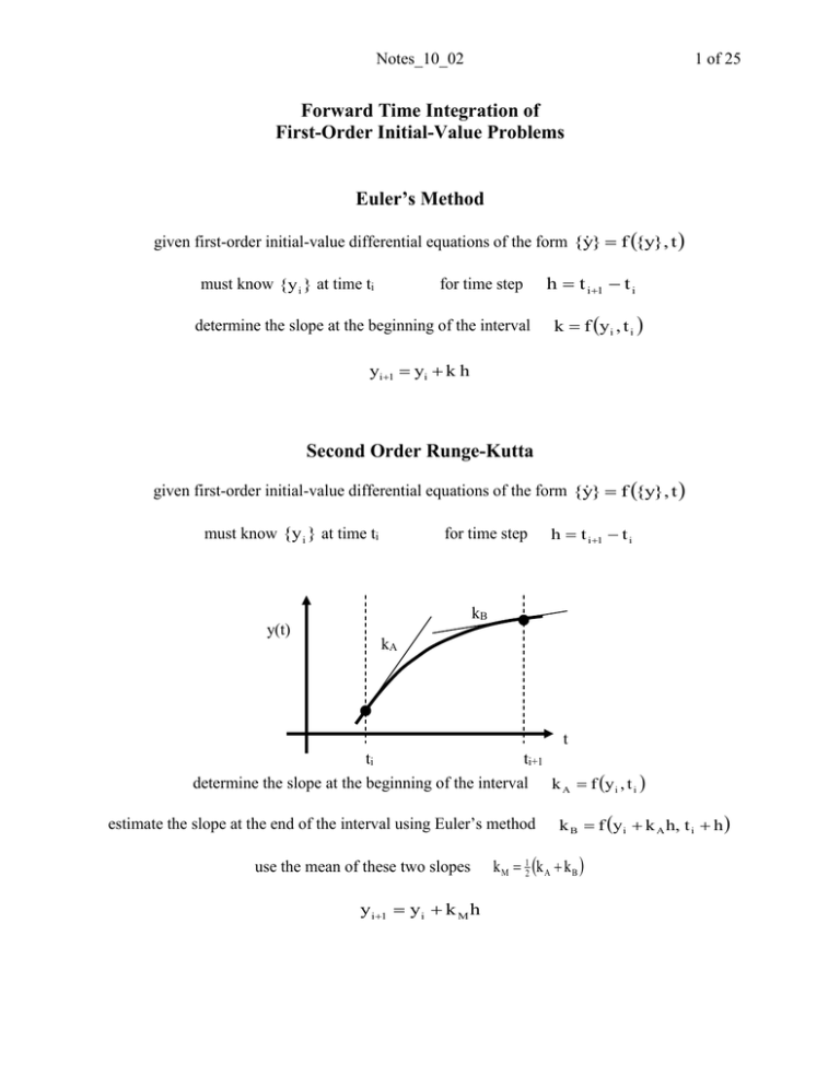
Second Order Runge-Kutta
 }  f {y}, t 
given first-order initial-value differential equations of the form {y
must know {y i } at time ti
for time step
h  t i 1  t i
kB
y(t)
kA
t
ti
ti+1
determine the slope at the beginning of the interval k A  f y i , t i 
estimate the slope at the end of the interval using Euler’s method
use the mean of these two slopes
y i 1  y i  k M h
k B  f y i  k A h, t i  h 
k M  12 k A  k B 
Notes_10_02
2 of 25
Fourth Order Runge-Kutta (RK4)
k4
k3
y(t)
k2
k1
t
ti
ti+½h
ti+1
determine the slope at the beginning of the interval
k1  f y i , t i 
estimate the slope at the midpoint of the interval using Euler’s method
k 2  f y i  k1 h2 , t i  h2 
estimate the slope at the midpoint of the interval using the new value
k 3  f y i  k 2 h2 , t i  h2 
estimate the slope at the end of the interval using the newest value
use a weighted mean of slopes
k 4  f y i  k 3 h , t i  h 
k M  16 k1  2k 2  2k 3  k 4 
y i 1  y i  k M h
Notes_10_02
3 of 25
Second-degree (Quadratic) Predictor and Third-degree (Cubic) Corrector
given first-order initial-value differential equations of the form {y
 }  f {y}, t 
must know {y}i , {y}i 1 , {y}i 2 respectively at times ti ti-1 and ti-2
 }i
may determine f i  {y
 }i 1
f i1  {y
= f(y,t)
 }i 2
f i 2  {y
fi
Note that the vertical axis
is y NOT y
fi-1
fi-2
ti-2
for fixed time step h
ti-1
ti
 = ( t - ti ) / h
ti+1
t
d = dt / h
dt = h d
fi
fi-1
fi-2
-2
-1
use second-degree polynomial predictor
 f i  1 0 0 a 0 
  
 
 f i 1   1  1 1  a 1 
f  1  2 4 a 
 i2  
 2 
0
+1

a 0 
 
f = a0 + a1  + a2 2 = 1    a 1 
a 
 2

2
a 0  2 0 0  f i 
  
 
 a 1   3  4 1  f i 1  / 2
a  1  2 1 f 
 2 
  i 2 

Notes_10_02
4 of 25
know coefficients a0, a1 and a2 for interpolant
yi+1 =

ti1
ti
f() = a0 + a1  + a2 2 = y ()
1
y dt + yi = h  f d  + yi = h ( a0 + a12 /2 + a23 /3 )
0
1
0
+ yi
yi+1 = yi + h ( a0 + a1 /2 + a2 /3 )
PREDICTOR (3-step Adams-Bashforth)
y i 1  y i  h23 f i  16 f i 1  5 f i 2  / 12
now use predicted value of yi+1 to compute f(yi+1) = fi+1*
fi
fi-1
fi+1*
fi-2
-2
use third-degree polynomial corrector
 f i*1  1 1
  
 f i  1 0
 
 f i 1  1  1
f i  2  1  2
1  b 0 
0 0   b1 
 
1  1 b 2 

4  8 b 3 
1
-1
0
b 0 
b 
1
f = b0 + b1  + b2 2 + b3 3 = [ 1  2 3 ] 
 
b 2 

b 3 

0
0   f i*1 
b 0   0 6
 b  2 3  6 1   
 1 
  f i  / 6
 
0   f i 1 
b 2  3  6 3

b 3  1  3 3  1 f i  2 
know coefficients b0, b1, b2 and b3 for new interpolant
yi+1 =

ti1
ti

+1
f() = b0 + b1  + b2 2 + b3 3 = y ()
1
y dt + yi = h  f d  + yi = h ( b0 + b12 /2 + b23 /3 + b34 /4 )
0
yi+1 = yi + h ( b0 + b1 /2 + b2 /3 + b3 /4 )
CORRECTOR (4-step Adams-Moulton)


y i1  y i  h 9 f i*1  19 f i  5 f i1  f i2 / 24
1
0
+ yi
Notes_10_02
variable time step second-degree polynomial predictor for f
0
0
 f i  1
 a 0 
a 0 
  

 
2 
 f i 1   1 ( t i 1  t i ) ( t i 1  t i )   a 1   [A] a 1 
f  1 ( t  t ) ( t  t ) 2  a 
a 
i 2
i
i 2
i
 i 2  
 2 
 2
yi+1 =

ti1
ti
5 of 25
f = a0 + a1 (t-ti) + a2 (t-ti)2
a 0 
 fi 
 

1 
 a 1   [A]  f i 1 
a 
f 
 2
 i 2 
y dt + yi
PREDICTOR
yi+1 = yi + a0 (ti+1-ti) + a1 (ti+1-ti)2 /2 + a2 (ti+1-ti)3 /3
use predicted value of yi+1 to compute f(yi+1,t) = fi+1*
use third-degree polynomial corrector for f
f i 1*  1 ( t i 1  t i ) ( t i 1  t i ) 2

 
0
0
 f i  1


2
 f i 1  1 ( t i 1  t i ) ( t i 1  t i )
 f  1 ( t i  2  t i ) ( t i  2  t i ) 2
 i2 
f = b0 + b1 (t-ti) + b2 (t-ti)2 + b3 (t-ti)3
( t i 1  t i ) 3  b 0 
b 0 
 
 
0
  b1   [B] b1 
( t i 1  t i ) 3  b 2 
b 2 
3 
b 3 
( t i  2  t i )  b 3 
f i 1* 
b 0 


b 
 1
1  f i 
   [B] 

b 2 
 f i 1 
b 3 
f 
 i2 
CORRECTOR
yi+1 = yi + b0 (ti+1-ti) + b1 (ti+1-ti)2 /2 + b2 (ti+1-ti)3 /3 + b3 (ti+1-ti)4 /4
FIXED TIME STEP
1) Predictor and corrector functions are constant coefficient, weighted sums of fi.
2) Coefficients are the same for all functions {y
 }  f {y}, t  .
VARIABLE TIME STEP
1) Matrices [A] and [B] must be inverted at each time step.
 }  f {y}, t  .
2) Matrices [A] and [B] are the same for all functions {y
Notes_10_02
6 of 25
Exact solution y = exp(-t)
1
0.5
0
0
0.1
0.2
0.3
0
-0.5
0.4
0.5
0.6
0.7
0.8
0.9
1
0.7
0.8
0.9
1
0.8
0.9
1
Predictor only - dt=0.001
x 10
-1
-1.5
0
0.1
0.2
-14
5
0.3
0.4
0.5
0.6
Predictor and Corrector - dt=0.001
x 10
Error
Error
-10
0
0
0.1
0.2
0.3
0.4
0.5
0.6
Time [sec]
0.7
Notes_10_02
% pred_corr.m - time integration using quadratic predictor, cubic corrector
%
simulate exponential y = exp(-t), ydot = -exp(-t) = -y
% HJSIII, 11.01.21
clear
% predictor-corrector coefficients
pred = [ 23 -16
5
] / 12;
corr = [ 9
19 -5 1 ] / 24;
% time step and duration of simulation
h = 0.001;
n = 1001;
nm1 = n - 1;
t = h * (0:nm1)';
% exact solution
y_exact = exp( -t );
% allocate space for solutions
y_pred_only = zeros(n,1);
f_pred_only = zeros(n,1);
y_pred_corr = zeros(n,1);
f_pred_corr = zeros(n,1);
% use exact solution for first three samples to get started
y_pred_only(1:3) = y_exact(1:3);
f_pred_only(1:3) = -y_pred_only(1:3);
y_pred_corr(1:3) = y_exact(1:3);
f_pred_corr(1:3) = -y_pred_corr(1:3);
% integrate forward in time
for i = 3 : nm1,
y_pred_only(i+1) = y_pred_only(i) ...
+ h * pred * [ f_pred_only(i) f_pred_only(i-1)
f_pred_only(i+1) = -y_pred_only(i+1);
f_pred_only(i-2) ]';
y_star = y_pred_corr(i) ...
+ h * pred * [ f_pred_corr(i) f_pred_corr(i-1) f_pred_corr(i-2) ]';
f_star = -y_star;
y_pred_corr(i+1) = y_pred_corr(i) ...
+ h * corr * [ f_star f_pred_corr(i) f_pred_corr(i-1) f_pred_corr(i-2) ]';
f_pred_corr(i+1) = -y_pred_corr(i+1);
end
% plot exact solution
figure( 1 )
clf
subplot( 3, 1, 1 )
plot( t,y_exact,'r' )
title( 'Exact solution
y = exp(-t)' )
% plot differences
err_pred_only = y_pred_only - y_exact;
err_pred_corr = y_pred_corr - y_exact;
subplot( 3, 1, 2 )
plot( t,err_pred_only,'g')
ylabel( 'Error' )
title( 'Predictor only - dt=0.001' )
subplot( 3, 1, 3 )
plot( t,err_pred_corr,'b' )
xlabel( 'Time [sec]' )
ylabel( 'Error' )
title( 'Predictor and Corrector - dt=0.001' )
% bottom of pred_corr
7 of 25
Notes_10_02
8 of 25
Forward Time Integration in MATLAB
[T,Y] = solver(odefun,tspan,y0)
[T,Y] = solver(odefun,tspan,y0,options)
odefun
A function handle that evaluates the right side of the differential equations. All
solvers solve systems of equations in the form y′ = f(t,y) or problems that involve a
mass matrix, M(t,y)y′ = f(t,y). The ode23s solver can solve only equations with
constant mass matrices. ode15s and ode23t can solve problems with a mass matrix
that is singular, i.e., differential-algebraic equations (DAEs).
tspan
A vector specifying the interval of integration, [t0,tf]. The solver imposes the
initial conditions at tspan(1), and integrates from tspan(1) to tspan(end). To
obtain solutions at specific times (all increasing or all decreasing), use tspan =
[t0,t1,...,tf].
For tspan vectors with two elements [t0 tf], the solver returns the solution
evaluated at every integration step. For tspan vectors with more than two elements,
the solver returns solutions evaluated at the given time points. The time values must
be in order, either increasing or decreasing.
Specifying tspan with more than two elements does not affect the internal time steps
that the solver uses to traverse the interval from tspan(1) to tspan(end). All solvers
in the ODE suite obtain output values by means of continuous extensions of the basic
formulas. Although a solver does not necessarily step precisely to a time point
specified in tspan, the solutions produced at the specified time points are of the same
order of accuracy as the solutions computed at the internal time points.
Specifying tspan with more than two elements has little effect on the efficiency of
computation, but for large systems, affects memory management.
y0
A vector of initial conditions.
options Structure of optional parameters that change the default integration
properties. This is the fourth input argument.
Notes_10_02
Solver
Problem
Type
Order of
Accuracy
9 of 25
When to Use
ode45
Nonstiff
Medium
Most of the time. This should be the first solver you
try.
ode23
Nonstiff
Low
For problems with crude error tolerances or for
solving moderately stiff problems.
ode113
Nonstiff
Low to high
For problems with stringent error tolerances or for
solving computationally intensive problems.
ode15s
Stiff
Low to
medium
If ode45 is slow because the problem is stiff.
ode23s
Stiff
Low
If using crude error tolerances to solve stiff systems
and the mass matrix is constant.
ode23t
Moderately
Stiff
Low
For moderately stiff problems if you need a solution
without numerical damping.
ode23tb
Stiff
Low
If using crude error tolerances to solve stiff systems.
Notes_10_02
10 of 25
MATLAB Algortihms
ode45
is based on an explicit Runge-Kutta (4,5) formula, the Dormand-Prince pair. It is a onestep solver – in computing y(tn), it needs only the solution at the immediately preceding time
point, y(tn-1). In general, ode45 is the best function to apply as a first try for most problems. [3]
ode23
is an implementation of an explicit Runge-Kutta (2,3) pair of Bogacki and Shampine. It
may be more efficient than ode45 at crude tolerances and in the presence of moderate stiffness.
Like ode45, ode23 is a one-step solver. [2]
ode113 is a variable order Adams-Bashforth-Moulton PECE solver. It may be more efficient
than ode45 at stringent tolerances and when the ODE file function is particularly expensive to
evaluate. ode113 is a multistep solver — it normally needs the solutions at several preceding
time points to compute the current solution. [7]
The above algorithms are intended to solve nonstiff systems. If they appear to be unduly slow,
try using one of the stiff solvers below.
ode15s
is a variable order solver based on the numerical differentiation formulas (NDFs).
Optionally, it uses the backward differentiation formulas (BDFs, also known as Gear's method)
that are usually less efficient. Like ode113, ode15s is a multistep solver. Try ode15s when
ode45 fails, or is very inefficient, and you suspect that the problem is stiff, or when solving a
differential-algebraic problem. [9], [10]
ode23s
is based on a modified Rosenbrock formula of order 2. Because it is a one-step solver, it
may be more efficient than ode15s at crude tolerances. It can solve some kinds of stiff problems
for which ode15s is not effective. [9]
ode23t
is an implementation of the trapezoidal rule using a "free" interpolant. Use this solver if
the problem is only moderately stiff and you need a solution without numerical damping. ode23t
can solve DAEs. [10]
ode23tb
is an implementation of TR-BDF2, an implicit Runge-Kutta formula with a first stage
that is a trapezoidal rule step and a second stage that is a backward differentiation formula of
order two. By construction, the same iteration matrix is used in evaluating both stages. Like
ode23s, this solver may be more efficient than ode15s at crude tolerances. [8], [1]
References
[1] Bank, R. E., W. C. Coughran, Jr., W. Fichtner, E. Grosse, D. Rose, and R.Smith, "Transient
Simulation of Silicon Devices and Circuits," IEEE Trans. CAD, 4 (1985), pp. 436–451.
[2] Bogacki, P. and L. F. Shampine, "A 3(2) pair of Runge-Kutta formulas," Appl. Math. Letters,
Vol. 2, 1989, pp. 321–325.
Notes_10_02
11 of 25
[3] Dormand, J. R. and P. J. Prince, "A family of embedded Runge-Kutta formulae," J. Comp.
Appl. Math., Vol. 6, 1980, pp. 19–26.
[4] Forsythe, G. , M. Malcolm, and C. Moler, Computer Methods for Mathematical
Computations, Prentice-Hall, New Jersey, 1977.
[5] Kahaner, D. , C. Moler, and S. Nash, Numerical Methods and Software, Prentice-Hall, New
Jersey, 1989.
[6] Shampine, L. F. , Numerical Solution of Ordinary Differential Equations, Chapman & Hall,
New York, 1994.
[7] Shampine, L. F. and M. K. Gordon, Computer Solution of Ordinary Differential Equations:
the Initial Value Problem, W. H. Freeman, SanFrancisco, 1975.
[8] Shampine, L. F. and M. E. Hosea, "Analysis and Implementation of TR-BDF2," Applied
Numerical Mathematics 20, 1996.
[9] Shampine, L. F. and M. W. Reichelt, "The MATLAB ODE Suite," SIAM Journal on
Scientific Computing, Vol. 18, 1997, pp. 1–22.
[10] Shampine, L. F., M. W. Reichelt, and J.A. Kierzenka, "Solving Index-1 DAEs in MATLAB
and Simulink," SIAM Review, Vol. 41, 1999, pp. 538–552.
Notes_10_02
12 of 25
spring-mass-damper with viscous damping using ODE23
1.5
Velocity [m/sec]
Position [m]
0.1
0.05
0
-0.05
-0.1
0
1
2
Time [sec]
3
1
0.5
0
-0.5
-1
-1.5
4
0
1
2
Time [sec]
3
4
Time step [msec]
25
20
15
mean time step = 17.05 msec
CPU time = 0.0466 sec
10
5
0
0
1
2
Time [sec]
3
4
spring-mass-damper with Coulomb friction using ODE23
Velocity [m/sec]
1.5
0.05
0
-0.05
-0.1
0
1
2
Time [sec]
3
4
1
0.5
0
-0.5
-1
-1.5
0
1
2
Time [sec]
3
4
40
Time step [msec]
Position [m]
0.1
30
mean time step = 9.4787 msec
CPU time = 0.2339 sec
20
10
0
0
1
2
Time [sec]
3
4
Notes_10_02
13 of 25
0.5
0.5
0.4
0.4
Velocity [m/sec]
Position [m]
drag-sled with Coulomb friction using ODE23
0.3
0.2
0.1
0
5
10
Time [sec]
0.1
15
Acceleration [m/s/s]
Time step [msec]
0.2
0
0
1500
1000
500
0
0.3
0
5
10
Time [sec]
15
0
5
10
Time [sec]
15
0
5
10
Time [sec]
15
2
0
-2
Notes_10_02
14 of 25
Second-Order Initial-Value Problems
Taylor Series Using Second Derivatives
given second-order initial-value differential equations of the form
 }  f {y}, t  and {y}  g{y},{y
 }, t 
{y
must know y i at time ti
may determine y i  f i and y i  g i
for time step
h  t i 1  t i
y i 1  y i  f i h  12 g i h 2
Fourth Order Runge-Kutta-Nystrom Using Second Derivatives (Fehlberg)
given second-order initial-value differential equations of the form
 }  f {y}, t  and {y}  g{y},{y
 }, t 
{y
must know y i at time ti
 i  f i and y i  g i
may determine y
k1  gy i , t i 




k 2  g y i  13 h f i  181 h 2 k 1 , t i  13 h
k 3  g y i  23 h f i  92 h 2 k 2 , t i  23 h

k 4  g y i  h f i  16 h 2 2k 1  k 3 , t i  h

1
y i 1  y i  h f i  120
h 2 13 k 1  36 k 2  9 k 3  2 k 4 
Notes_10_02
15 of 25
Fifth-degree (Quintic) Predictor and Seventh-degree (Heptic) Corrector
with Second Derivatives
given second-order initial-value differential equations of the form
 }  f {y}, t  and {y}  g{y},{y
 }, t 
{y
must know {y}i , {y}i1 , {y}i2 respectively at times ti, ti-1 and ti-2
 }i , {y
 }i 1 , {y
 }i2 and {y}i , {y}i1 , {y}i2
may determine {y
= f(y)
fi
gi
fi-1
gi-1
fi-2
gi-2
ti-2
fixed time step h
ti-1
 = ( t - ti ) / h
ti
ti+1
d = dt / h
fi-1
gi-1
t
dt = h d
d /dt = 1 / h
fi
gi
fi-2
gi-2
-2
-1
use fifth degree polynomial predictor
g
df
f d

dt
 dt
gh
f

0
+1

f  a 0  a 1  a 2  2  a 3  3  a 4  4  a 5  5
g h  a 1  2a 2   3a 3  2  4a 4  3  5a 5  4
Notes_10_02
 f  1   2  3
 
2
g h  0 1 2 3
4
4 3
16 of 25
a 0 
a 
 1
5
 
a 2 



4 
5  a 3 
a 4 
 

a 5 

0
0
0
0  a 0 
 f i  1 0

 f
 1  1 1  1
1
 1  
a 1 
 i 1  

 f i2 
 1  2 4  8 16  32 
a 2 



 
a
g
h
0
1
0
0
0
0
 i  
 3 
 g i 1 h  0 1  2 3
4
5  a 4 

 
 

g i  2 h 
 0 1  4 12  32 80  
a 5 

0 0 0 0 0  f i 
a 0   4
a   0

0 0 4 0 0 
 1 
 f i 1 

a 2 
  23 16 7 12 16 2 
 f i2 

 

/ 4
a 3    33 16 17 13 32 5  g i h 
a 4    17 4 13 6 20 4  g i 1 h 
  



g i  2 h 

a 5 
   3 0 3 1 4 1 
know coefficients ai for interpolant
y i1  
ti1
ti
1
f   a 0  a 1  a 2  2  a 3  3  a 4  4  a 5  5  y 

y dt  y i  h  f d  y i  y i  h a 0   a 1 2 / 2  a 2 3 / 3  a 3  4 / 4  a 4 5 / 5  a 5  6 / 6
0
y i1  y i  ha 0  a 1 / 2  a 2 / 3  a 3 / 4  a 4 / 5  a 5 / 6
PREDICTOR (3-step Obreshkov)
y  y i  h  949 f i  608 f i1  581 f i2  h 637 g i  1080 g i1  173 g i2  / 240
*
i 1

1
0
Notes_10_02
now use predicted value of
17 of 25
 
y *i 1 to compute f y*i1  f i*1 and gy *i1   g *i1
fi-1
gi-1
fi
gi
fi+1*
gi+1*
fi-2
gi-2
-2
-1
0
+1

use seventh degree polynomial corrector
f   b 0  b1  b 2  2  b 3  3  b 4  4  b 5  5  b 6  6  b 7  7  y 
 f  1   2  3
 
2
g h  0 1 2 3
4
4 3
5
5 4
6
6 5
b 0 
b 
 1
b 2 
 
 7  b 3 
 
7  6  b 4 
b 5 
 
b 6 
b 
 7
 f i*1  1 1
1
1
1
1
1
1  b 0 

 

0
0
0
0
0
0  
 f i  1 0
 b1 
 f i 1  1  1 1  1
1
1
1
 1  b 2 

 
 
64
 128 b 3 
 f i  2  1  2 4  8 16  32
 * 
 
2
3
4
5
6
7  b 4 
 g i 1  0 1

 g i  0 1
0
0
0
0
0
0  b 5 

 
 
4
5
6
7  b 6 
 g i 1  0 1  2 3

g  0 1  4 12  32 80  192 448  b 
 7 
 i2  
Notes_10_02
18 of 25
108
0
0
0
0
0
01   f i*1 
b 0   0


b   0
0
0
0
0
108
0
0   f i 
 1 
b 2   56  297 216
25  12 108
108
6   f i 1 

  

0
3   f i2 
b 3   124  27  108 11  24  189
/ 108
 
  g *i 1 
b
50
270

270

50

3

216

189

12
4
  


b 5   59
54
27
 22 21
54
 27  6   g i 
  


108
25
15
108
81
6   g i 1 
b 6   52  81

b    11  27

27
11
3
27
27
3
 
 7 
g i  2 
f   b 0  b1  b 2  2  b 3  3  b 4  4  b 5  5  b 6  6  b 7  7  y 
know coefficients bi
y i 1  
ti1
ti

1
y dt  y i  h  f d  y i
0
 y i  h b 0   b1  / 2  b 2  3 / 3  b 3  4 / 4  b 4  5 / 5  b 5  6 / 6  b 6  7 / 7  b 7  8 / 8
2
y i1  y i  hb 0  b1 / 2  b 2 / 3  b 3 / 4  b 4 / 5  b 5 / 6  b 6 / 7  b 7 / 8
CORRECTOR (4-step Obreshkov)
y i 1
 34465 f i*1  42255 f i  12015 f i 1  1985 f i  2
 yi  h 
  h  3849 g *  22977 g  7263 g  489 g
i 1
i
i 1
i2



 / 90720




1
0
Notes_10_02
19 of 25
Third-degree (Cubic) Predictor and Third-degree (Cubic) Corrector
with Second Derivatives
given second-order initial-value differential equations of the form
 }  f {y}, t  and {y}  g{y},{y
 }, t 
{y
must know {y}i and {y}i1 respectively at times ti and ti-1
may determine {y }i {y }i1 and {y}i {y}i
= f(y)
ti-1
fixed time step h
fi
gi
fi-1
gi-1
 = ( t - ti ) / h
ti
d = dt / h
-1
0
use third degree polynomial predictor
df
f d

dt
 dt
gh
t
dt = h d
d /dt = 1 / h
fi
gi
fi-1
gi-1
g
ti+1
f

+1

f  a 0  a 1  a 2  2  a 3  3
g h  a 1  2a 2   3a 3  2
a 0 
 
 a 1 
 f  1  

  

2 
g h  0 1 2 3  a 2 

a 3 

2
3
Notes_10_02
20 of 25
0
0  a 0 
 f i  1 0
 f
 1  1 1  1  a 
 i 1  
1



 


a
g
h
0 1
0
0  2
 i 




g i 1 h  0 1  2 3  
a 3 

a 0   1
a   0
 1 
 
a 2    3


a 3 
  2
0 0 0  f i 

0 1 0 
 f i 1 


3 2 1  g i h 

2 1 1 
g i 1 h 

know coefficients ai for interpolant
y i1  
ti1
ti
f   a 0  a 1   a 2  2  a 3  3  y 

1
y dt  y i  h  f d  y i  y i  h a 0   a 1 2 / 2  a 2 3 / 3  a 3  4 / 4
0
y i1  y i  ha 0  a 1 / 2  a 2 / 3  a 3 / 4
PREDICTOR (2-step Obreshkov per Sehnalova)
y*i1  y i  h  6 f i  18 f i1  h 17 g i  7g i1  / 12
now use predicted value of
 
y *i 1 to compute f y*i1  f i*1 and gy *i1   g *i1
fi
gi
0
use third degree polynomial corrector
fi+1*
gi+1*
+1

f   b 0  b1   b 2  2  b 3  3  y 
b 0 
 
 f  1   2  3   b1 
 

2 
g h  0 1 2 3  b 2 

b 3 


1
0
Notes_10_02
 f i 1  1
 f  1
 i  


g i 1 h  0


 gi h 
 0
21 of 25
1 1 1  b 0 

0 0 0 
 b1 
 
1 2 3 b 2 

1 0 0 
b 3 

1
0
0   f i 1 
b 0   0
b   0

0
0
1  
 1 
 fi 

 


b 2   3  3  1  2 g i 1 h 



1
1 
 gi h 

b 3 
  2 2
know coefficients bi
y i 1  
ti1
ti

f   b 0  b1   b 2  2  b 3  3  y 
y dt  y i  h
1

0
f d  y i
 y i  h b 0   b1  2 / 2  b 2  3 / 3  b 3  4 / 4

1
0
y i1  y i  hb 0  b1 / 2  b 2 / 3  b 3 / 4
CORRECTOR (2-step Obreshkov per Sehnalova)
y*i1  y i  h 6 f i1  6 f i  h  g i1  g i  / 12
Notes_10_02
22 of 25
Least-Squares Quadratic Predictor and Cubic Corrector
with Second Derivatives
given second-order initial-value differential equations of the form
 }  f {y}, t  and {y}  g{y},{y
 }, t 
{y
must know {y}i , {y}i1 , {y}i2 respectively at times ti, ti-1 and ti-2
may determine {y }i , {y }i1 , {y }i2 and {y}i , {y}i1 , {y}i2
= f(y)
fi
fi-1
fi-2
ti-2
fixed time step h
ti-1
 = ( t - ti ) / h
ti
ti+1
d = dt / h
t
dt = h d
d /dt = 1 / h
fi
fi-1
fi-2
-2
-1
0
+1
use quadratic polynomial predictor
g
df f d

dt  dt

f = a0 + a1  + a2 2
g  a 1  2a 2   / h
a 0 
 f  1  2   
 
  a1 
g h  0 1 2 a 
 2
g h  a 1  2a 2 
Notes_10_02
23 of 25
0 
 f i  1 0
 g h  0 1
0 
 i  
a 0 

 f i 1 
 1  1 1   


a 1 
 g i 1 h  0 1  2 a 
 f i  2  1  2 4   2 

 


g i  2 h 
 0 1  4
 fi 
g h
 i 
 f

Y   i1 
 g i 1 h 
 f i2 



g i 2 h 

Y  X
  XT X XT Y
1
0
1 0
0 1
0 

1  1 1 
X  

0 1  2 
1  2 4 


0 1  4
a 0 
   a 1 
a 
 2
least squares solution
 fi 
g h
16   i 
a 0   71 36 40 26 19
  
 f i 1 


 a 1   36 86  20 26  16  34 
 / 130
g i 1 h 
a   5 30  10 0

5
 30
 2 
 f i2 


g i  2 h 


know coefficients a0, a1 and a2 for interpolant
yi+1 =

ti1
ti
f() = a0 + a1  + a2 2 = y ()
1
y dt + yi = h  f d  + yi = h ( a0 + a12 /2 + a23 /3 )
0
1
0
+ yi
yi+1 = yi + h ( a0 + a1 /2 + a2 /3 )
PREDICTOR (least-squares 3-step Adams-Bashforth)
y i 1  y i  h 272 f i  80 f i 1  38 f i 2  h 267 g i  117 g i 1  33 g i 2  / 390
Notes_10_02
24 of 25
now use predicted value of yi+1 to compute f(yi+1) = fi+1* and g(yi+1) = gi+1*
fi
fi-1
fi+1*
fi-2
-2
-1
use cubic polynomial corrector
0
+1

f = b0 + b1  + b2 2 + b3 3
b 0 
 
 f  1   2  3   b1 
 

2 
g h  0 1 2 3  b 2 

b 3 

 f i*1  1 1
1
1
 *  
2
3 
g i 1 h  0 1
 f i  1 0
0
0  b 0 

 

0
0   b1 
 g i h  0 1


 
f
i

1

 1  1 1  1 b 2 
g i 1 h  0 1  2 3  b 3 

 

 f i  2  1  2 4  8
g h  0 1  4 12 

 i 1  
 f i*1 
 * 
g i 1 h 
542
374
241 159   f i 
b 0   754  438 851 175


 b   590 126
175
593  374 394  391  471  g i h 
 1 
 

 / 2388
618  203  67
4
 266 167
21   f i 1 
b 2   32

b 3   45 213  69  111 69
 111 45
213  g i 1 h 


 f i2 
g h 
 i 1 
know coefficients b0, b1, b2 and b3 for new interpolant
f() = b0 + b1  + b2 2 + b3 3 = y ()
Notes_10_02
yi+1 =

ti1
ti
25 of 25
1
y dt + yi = h  f d  + yi = h ( b0 + b12 /2 + b23 /3 + b34 /4 )
0
1
0
yi+1 = yi + h ( b0 + b1 /2 + b2 /3 + b3 /4 )
CORRECTOR (least-squares 4-step Adams-Moulton)
y i 1
12581 f i*1  10243 f i  4483 f i 1  1349 f i  2
 yi  h 
  h  1389 g *  5057 g  5455 g  195 g
i 1
i
i 1
i2


does not work as well as Obreshkov

 / 28656



+ yi