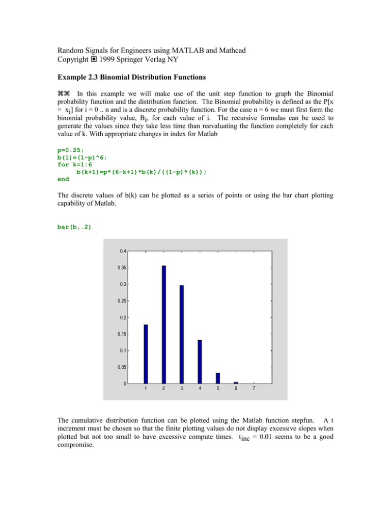
Random Signals for Engineers using MATLAB and Mathcad
Copyright  1999 Springer Verlag NY
Example 2.3 Binomial Distribution Functions
In this example we will make use of the unit step function to graph the Binomial
probability function and the distribution function. The Binomial probability is defined as the P[x
= xi] for i = 0 .. n and is a discrete probability function. For the case n = 6 we must first form the
binomial probability value, Bi, for each value of i. The recursive formulas can be used to
generate the values since they take less time than reevaluating the function completely for each
value of k. With appropriate changes in index for Matlab
p=0.25;
b(1)=(1-p)^6;
for k=1:6
b(k+1)=p*(6-k+1)*b(k)/((1-p)*(k));
end
The discrete values of b(k) can be plotted as a series of points or using the bar chart plotting
capability of Matlab.
bar(b,.2)
0.4
0.35
0.3
0.25
0.2
0.15
0.1
0.05
0
1
2
3
4
5
6
7
The cumulative distribution function can be plotted using the Matlab function stepfun. A t
increment must be chosen so that the finite plotting values do not display excessive slopes when
plotted but not too small to have excessive compute times. tinc = 0.01 seems to be a good
compromise.
t=0:.01:6.9;
t0=1:7;
plot(bin_dist(b,t,t0))
1
0.9
0.8
0.7
0.6
0.5
0.4
0.3
0.2
0.1
0
0
100
200
300
400
500
600
700
The following functions are defined:
function y=bin_dist(b,t,t0)
% BIN_DIST is the cumulative distribution for a
% binomial distribution where b = vector probabilites
% t = time vector and t0 is where the steps take place
% b and t0 must be the same length
k=length(b);
y=zeros(1,length(t));
for i=1:k
y = b(i)*stepfun(t,t0(i))+y;
end
function y=stepfun(t,t0)
% stepfun
y =(t>t0);
