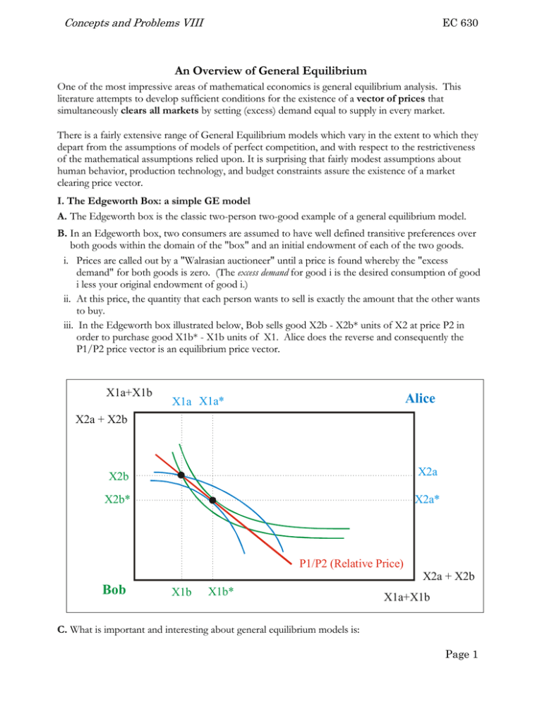
Concepts and Problems VIII
EC 630
An Overview of General Equilibrium
One of the most impressive areas of mathematical economics is general equilibrium analysis. This
literature attempts to develop sufficient conditions for the existence of a vector of prices that
simultaneously clears all markets by setting (excess) demand equal to supply in every market.
There is a fairly extensive range of General Equilibrium models which vary in the extent to which they
depart from the assumptions of models of perfect competition, and with respect to the restrictiveness
of the mathematical assumptions relied upon. It is surprising that fairly modest assumptions about
human behavior, production technology, and budget constraints assure the existence of a market
clearing price vector.
I. The Edgeworth Box: a simple GE model
A. The Edgeworth box is the classic two-person two-good example of a general equilibrium model.
B. In an Edgeworth box, two consumers are assumed to have well defined transitive preferences over
both goods within the domain of the "box" and an initial endowment of each of the two goods.
i. Prices are called out by a "Walrasian auctioneer" until a price is found whereby the "excess
demand" for both goods is zero. (The excess demand for good i is the desired consumption of good
i less your original endowment of good i.)
ii. At this price, the quantity that each person wants to sell is exactly the amount that the other wants
to buy.
iii. In the Edgeworth box illustrated below, Bob sells good X2b - X2b* units of X2 at price P2 in
order to purchase good X1b* - X1b units of X1. Alice does the reverse and consequently the
P1/P2 price vector is an equilibrium price vector.
X1a+X1b
Alice
X1a X1a*
X2a + X2b
X2b
X2a
X2b*
X2a*
P1/P2 (Relative Price)
X2a + X2b
Bob
X1b
X1b*
X1a+X1b
C. What is important and interesting about general equilibrium models is:
Page 1
Concepts and Problems VIII
EC 630
i. All markets are modelled simultaneously, so if an equilibrium exists all markets also “clear”
simultaneously.
ii. GE models make it clear that “every thing comes from some where,” which is the core assumption
to the “no free lunches” claim that economists often make.
iii. GE models of competitive markets can also prove that it is possible to clear all markets
simultaneously, a claim that is not intuitively obvious.
a. That such equilibria can be proven to exist in very general models is also somewhat remarkable.
b. Typical assumptions for the classic models are developed below.
iv. GE models of competitive models can also prove that the equilibria (there may be more than one)
are Pareto efficient, which is an important part of the economists normative case for competitive
markets.
D. Weaknesses of the GE model
i. In spite of the strength of GE analysis, there are a number of weaknesses as well.
ii. For example, although existence can be proved, it cannot be proven that an equilibrium will
emerge spontaneously via “invisible hand” processes (as argued by Adam Smith and Walras).
iii. The classic models make rather strong assumptions about information (everyone knows all prices
and their tastes) and the lack of disequilibrium trades (only the equilibrium is modeled).
iv. The normative claims also ignore the presence (necessity) of government and externalities. (All
property rights are assumed to be perfectly defined and all property tradable, and no externalities
problems exist.)
a. These can be added to the models, but are not done so routinely.
b. The existence of externalities and transactions costs would weaken many of the normative
conclusions:
v. There are also issues about the empirical relevance of the models: is there really a stable
equilibrium in the real world, or is the GE model simply a rough model tha helps us understand
even more complex economic relationships?
vi. However, even granting all the weaknesses, it bears noting that the models are important
contributions to the theoretical literature and many contemporary macroeconomists (and
macroeconomic theories) use computable forms of GE models in their analyses and empirical
work.
II. An Example of a General Competitive Model
A. Typical assumptions of a general competitive model (without production):
i. Goods:
a. Goods are characterized by time location and state of the world.
b. There are assumed to be a finite number of goods, k.
c. Agent i's consumption bundle is denoted xi and is a k-dimensioned vector of the goods possessed
by i.
d. The amount of the jth good possessed by individual i is denoted xij.
e. An individual's initial endowment of good is his "pre trade" consumption bundle, wi.
f. An allocation of goods is a vector describing each individual's consumption bundle, x = [ x1, x2,
... xn ]
Page 2
Concepts and Problems VIII
EC 630
g. A feasible allocation for the economy is one that is possible. In the pure exchange case of interest
here, it is one where xi = wi. (A feasible allocation is one in which the total consumption of
each good equals the economy wide initial endowment of that good.)
ii. Agents:
a. Each consumer i is described by a complete transitive preference ordering >i (which is used to
derive a utility function Ui) and an initial endowment wi.
b. Each consumer is a utility maximizing price taker.
c. Thus each consumer maximizes Ui(xi) s. t. Pxi = Pwi (P is a 1xk vector, and wi and xi are kx1
vectors.)
d. (In a model with production, there will also be k production functions which describe how
"inputs" can be transformed into "final consumption goods.")
iii. A Walrasian equilibrium in a barter economy is said to exist if price vector P* exists such that 
xi(P*, P*wi)  wi  where function xi is vector representing the utility maximizing levels of all
goods for individual i with initial endowment wi. That is to say when a price vector exists such that
demand is less than or equal to supply in every market.
B. Some Properties of the Model
i. The budget set is homogeneous of degree 0 in prices. If you multiply all prices by any constant k,
there is no change in an individual's budget constraint.
a. This implies that the demand correspondence xi is also homogeneous in all prices. E.g. there is
no money illusion.
b. The excess demand function ( xi(P, Pwi) - wi ) is for the same reason also homogeneous in all
prices.
c. Moreover, since the sum of homogeneous functions of degree k is also homogeneous of degree
k, the excess demand function is homogeneous of degree 0 in prices.
ii. Individual i's excess demand for good i is simply his ordinary demand for good j (his desired
consumption) less his initial endowment, zij(P) = xij(P,Pwij) - wij .
iii. Each individual i's vector of desired consumption is determined in the usual way -- by maximizing
individual i's utility subject to his budget constraint.
iv. The vector of aggregate excess demand is written as z(P) =  ( xi(P, Pwi) - wi )
C. Walras Law. (Varian's version) For any P in Sk (remember there are k goods) excess aggregate
demand (in dollars) is zero, that is P z(P) = 0. (Sk is the commodity space.)
i. Proof: recall that z(P) =  ( xi(P, Pwi) - wi ), and also that each person's demand correspondence
(vector xi) is derived by maximizing utility given a budget constraint. Consequently, Pwi = Pxi for
each individual. This implies that the sum of all Pwi has to equal the sum of all Pxi. That is to say,
excess demand is always zero in the aggregate (measured by the numeraire good, here dollars).
D. Note that the above implies that if P* is a Walrasian equilibrium and excess demand for
commodity j is less than zero, zj(P*) 0, then P*j = 0. (If there is an excess supply of good j ,
then its price has to be zero.)
i. Proof: Since P* is a Walrasian Equilibrium the excess demand for all goods is less than or equal to
zero, it satisfies z(P*)  0. If P*j were greater than zero then P*j z(P*) < 0, violating Walras' law.
But Walras' law always holds, so P*j has to be zero.
Page 3
Concepts and Problems VIII
EC 630
E. Similarly, if all goods are desirable at the margin and P* is a Walrasian equilibrium, then
z(P*) =
0.
i. In this case, excess demand is zero in every market. (Supply equals demand in all markets.)
ii. The proof is left as an exercise. It is very similar to the previous case.
F. Moreover, (usual version of Walras Law) if K-1 markets have cleared, jk-1 zj(P)=0, then (Varian's
version and Ci) Walras' law imply that the kth market must also have cleared,
e. g. pkzk(P) = 0.
G. Summary:
i. The aggregate value of excess demand is always zero.
ii. If there is an excess supply of a good (an undesirable good) its price will be zero.
iii. Otherwise, demand equals supply in Walrasian equilibrium for all goods.
III. Proof of the Existence of a Walrasian Equilibrium (based on Varian’s proof)
A. Browers Fixed Point Theorem. If f:Sk-1  Sk-1 is continuous function from the unit simplex to itself,
there exists some x in Sk-1 such that x = f(x). Such a point is called a fixed point.
i. In a one dimensional case, the unit simplex is just the 0-1 closed interval.
ii. (In the two dimensional case it is a 1x1 square, in the three dimensional case it is a 1x1x1 cube,
etc.)
iii. To see that a function from this interval to all or part of itself has a fixed point, draw diagram of a
function, Y = f(x). Let Y be the vertical axis, X be the horizontal axis. A continuous function goes
from [0-1] on the horizontal axis to some part of [0-1] on the vertical axis. Because of continuity,
at some point the function will intersect the 45o line from (0,0) to (1,1), at which point x* = f(x*).
Such a point, x*, is said to be a fixed point. (There may be more than one fixed point for a given
function.)
B. The ingeneous trick in most existence proofs is to construct a transformation based on the choice
setting that is a continuous function mapping of the variables of interest into themselves, here
prices.
C. One example of such a mapping is the following:
i. define map g : Sk-1  Sk-1 by gj(P) = [Pj + max (0, zj(P) ] / [1 + jk max (0, Zj(P)]
ii. where the prices have been normalized as: Pj = Pj/Pn (This of course will not affect aggregate
demand as we have already established above.)
iii. This map is continuous since z and max (0, zj(p)) are continuous.
iv. It lies in the unit simplex since gi = 1.
v. By Browers fixed point theorem there is a P* such that P*j = gj(P*) for all j. (That is to say a fixed
point exists.)
vi. Thus Pj* = [Pj* + max (0, zj(P*) ] / [1 + jk max (0, zj(P*)]
D. P* turns out to be a Walrasian equilibrium price vector.
i. Cross multiplying yields Pj* [1 + n max (0, zn(P*)]= [Pj* + max (0, zj(P*) ]
ii. Then Multiplying both sides by zi(P*)
zj(P*)Pj* [1 + jk max (0, zj(P*)]= zj(P*)[Pj* + max (0, zj(P*) ]
iii. Adding these up across all goods:
jzj(P*)Pj* ][1 + jk max (0, zn(P*)]= jzj(P*)[Pj* + max (0, zj(P*) ]
Page 4
Concepts and Problems VIII
EC 630
iv. From Walras law we know that the left-hand side equals zero. (The first term in brackets terms
has to be zero.)
v. If the right hand side equals zero, zj(P*) has to be zero for all j. (Otherwise, the product of zj(P*)[Pj*
+ max (0, zj(P*) ] would exceed zero. Q. E. D.
E. The economic meaning of this existance proof is that a market clearing price vector exists. That is
to say, given the usual assumptions about preferences (and in a more general model, production
correspondences) a price vector exists that simulaneously clears all markets. At this price vector,
(a) the excess demand for all goods (things with P>0) is zero, and (b) all tradable "things" with
negative excess demand have zero prices.
IV. Review Problem
A. Work through an existence proof for a two dimensional Edgeworth box. That is to say formally
lay out your assumptions and work through a two dimensional version of the proof outlined
above.
B. Critique the Walrasian model. To some extent the above existence proof looks very general.
Think a bit about the assumptions and see if you can find any implicit or explicit assumptions
which are unbelievable.
Page 5