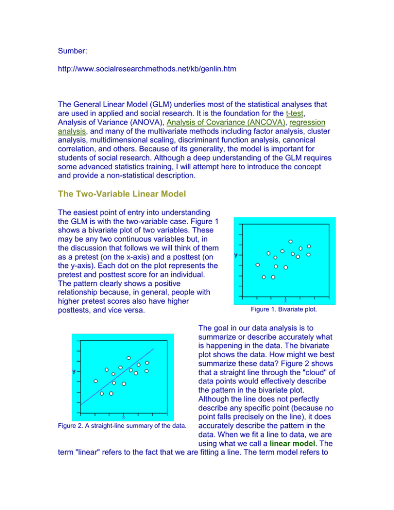
Sumber:
http://www.socialresearchmethods.net/kb/genlin.htm
The General Linear Model (GLM) underlies most of the statistical analyses that
are used in applied and social research. It is the foundation for the t-test,
Analysis of Variance (ANOVA), Analysis of Covariance (ANCOVA), regression
analysis, and many of the multivariate methods including factor analysis, cluster
analysis, multidimensional scaling, discriminant function analysis, canonical
correlation, and others. Because of its generality, the model is important for
students of social research. Although a deep understanding of the GLM requires
some advanced statistics training, I will attempt here to introduce the concept
and provide a non-statistical description.
The Two-Variable Linear Model
The easiest point of entry into understanding
the GLM is with the two-variable case. Figure 1
shows a bivariate plot of two variables. These
may be any two continuous variables but, in
the discussion that follows we will think of them
as a pretest (on the x-axis) and a posttest (on
the y-axis). Each dot on the plot represents the
pretest and posttest score for an individual.
The pattern clearly shows a positive
relationship because, in general, people with
higher pretest scores also have higher
posttests, and vice versa.
Figure 1. Bivariate plot.
The goal in our data analysis is to
summarize or describe accurately what
is happening in the data. The bivariate
plot shows the data. How might we best
summarize these data? Figure 2 shows
that a straight line through the "cloud" of
data points would effectively describe
the pattern in the bivariate plot.
Although the line does not perfectly
describe any specific point (because no
point falls precisely on the line), it does
Figure 2. A straight-line summary of the data.
accurately describe the pattern in the
data. When we fit a line to data, we are
using what we call a linear model. The
term "linear" refers to the fact that we are fitting a line. The term model refers to
the equation that summarizes the line that we fit. A line like the one shown in
Figure 2 is often referred to as a regression line and the analysis that produces
it is often called
regression
analysis.
Figure 3 shows the
equation for a
straight line. You
may remember this
equation from your
high school algebra
classes where it is
often stated in the
form y = mx + b. In
this equation, the
components are:
Figure 3. The straight-line model.
y = the y-axis
variable, the
outcome or posttest
x = the x-axis variable, the pretest
b0 = the intercept (value of y when x=0)
b1 = the slope of the line
The slope of the line is the change in the posttest given in pretest units. As
mentioned above, this equation does not perfectly fit the cloud of points in Figure
1. If it did, every point would fall on the line. We need one more component to
describe the way this line is fit to the bivariate plot.
Figure 4 shows the
equation for the two
variable or bivariate
linear model. The
component that we
have added to the
equation in Figure 3
is an error term, e,
that describes the
vertical distance
from the straight line
to each point. This
Figure 4. The two-variable linear model.
term is called "error"
because it is the
degree to which the line is in error in describing each point. When we fit the twovariable linear model to our data, we have an x and y score for each person in
our study. We input these value pairs into a computer program. The program
estimates the b0 and b1 values for us as indicated in Figure 5. We will actually get
two numbers back that
are estimates of those
two values.
You can think of the
two-variable regression
line like any other
descriptive statistic -- it
is simply describing the
relationship between
two variables much as
a mean describes the
central tendency of a
Figure 5. What the model estimates.
single variable. And,
just as the mean does
not accurately represent every value in a distribution, the regression line does not
accurately represent every value in the bivariate distribution. We use these
summaries because they show the general patterns in our data and allow us to
describe these patterns in more concise ways than showing the entire distribution
allows.
The General Linear Model
Given this brief introduction to the two-variable case, we are able to extend the
model to its most general case. Essentially the GLM looks the same as the two
variable model shown in Figure 4 -- it is just an equation. But the big difference is
that each of the four terms in the GLM can represent a set of variables, not just a
single one. So, the general linear model can be written:
y = b0 + bx + e
where:
y = a set of outcome variables
x = a set of pre-program variables or covariates
b0 = the set of intercepts (value of each y when each x=0)
b = a set of coefficients, one each for each x
You should be able to see that this model allows us to include an enormous
amount of information. In an experimental or quasi-experimental study, we would
represent the program or treatment with one or more dummy coded variables,
each represented in the equation as an additional x-value (although we usually
use the symbol z to indicate that the variable is a dummy-coded x). If our study
has multiple outcome variables, we can include them as a set of y-values. If we
have multiple pretests, we can include them as a set of x-values. For each xvalue (and each z-value) we estimate a b-value that represents an x,y
relationship. The estimates of these b-values, and the statistical testing of these
estimates, is what enables us to test specific research hypotheses about
relationships between variables or differences between groups.
The GLM allows us to summarize a wide variety of research outcomes. The
major problem for the researcher who uses the GLM is model specification.
The researcher is responsible for specifying the exact equation that best
summarizes the data for a study. If the model is misspecified, the estimates of
the coefficients (the b-values) are likely to be biased (i.e., wrong) and the
resulting equation will not describe the data accurately. In complex situations,
this model specification problem can be a serious and difficult one (see, for
example, the discussion of model specification in the statistical analysis of the
regression-discontinuity design).
The GLM is one of the most important tools in the statistical analysis of data. It
represents a major achievement in the advancement of social research in the
twentieth century.