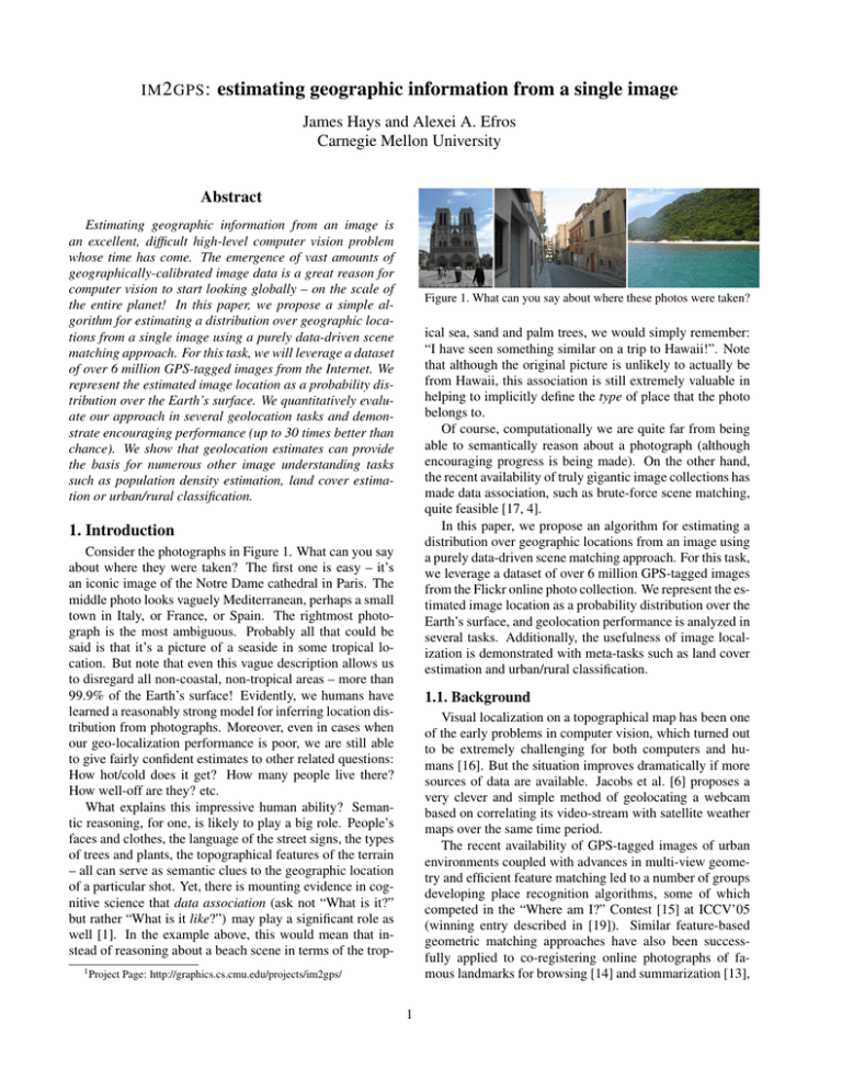
IM 2 GPS :
estimating geographic information from a single image
James Hays and Alexei A. Efros
Carnegie Mellon University
Abstract
Estimating geographic information from an image is
an excellent, difficult high-level computer vision problem
whose time has come. The emergence of vast amounts of
geographically-calibrated image data is a great reason for
computer vision to start looking globally – on the scale of
the entire planet! In this paper, we propose a simple algorithm for estimating a distribution over geographic locations from a single image using a purely data-driven scene
matching approach. For this task, we will leverage a dataset
of over 6 million GPS-tagged images from the Internet. We
represent the estimated image location as a probability distribution over the Earth’s surface. We quantitatively evaluate our approach in several geolocation tasks and demonstrate encouraging performance (up to 30 times better than
chance). We show that geolocation estimates can provide
the basis for numerous other image understanding tasks
such as population density estimation, land cover estimation or urban/rural classification.
Figure 1. What can you say about where these photos were taken?
ical sea, sand and palm trees, we would simply remember:
“I have seen something similar on a trip to Hawaii!”. Note
that although the original picture is unlikely to actually be
from Hawaii, this association is still extremely valuable in
helping to implicitly define the type of place that the photo
belongs to.
Of course, computationally we are quite far from being
able to semantically reason about a photograph (although
encouraging progress is being made). On the other hand,
the recent availability of truly gigantic image collections has
made data association, such as brute-force scene matching,
quite feasible [17, 4].
In this paper, we propose an algorithm for estimating a
distribution over geographic locations from an image using
a purely data-driven scene matching approach. For this task,
we leverage a dataset of over 6 million GPS-tagged images
from the Flickr online photo collection. We represent the estimated image location as a probability distribution over the
Earth’s surface, and geolocation performance is analyzed in
several tasks. Additionally, the usefulness of image localization is demonstrated with meta-tasks such as land cover
estimation and urban/rural classification.
1. Introduction
Consider the photographs in Figure 1. What can you say
about where they were taken? The first one is easy – it’s
an iconic image of the Notre Dame cathedral in Paris. The
middle photo looks vaguely Mediterranean, perhaps a small
town in Italy, or France, or Spain. The rightmost photograph is the most ambiguous. Probably all that could be
said is that it’s a picture of a seaside in some tropical location. But note that even this vague description allows us
to disregard all non-coastal, non-tropical areas – more than
99.9% of the Earth’s surface! Evidently, we humans have
learned a reasonably strong model for inferring location distribution from photographs. Moreover, even in cases when
our geo-localization performance is poor, we are still able
to give fairly confident estimates to other related questions:
How hot/cold does it get? How many people live there?
How well-off are they? etc.
What explains this impressive human ability? Semantic reasoning, for one, is likely to play a big role. People’s
faces and clothes, the language of the street signs, the types
of trees and plants, the topographical features of the terrain
– all can serve as semantic clues to the geographic location
of a particular shot. Yet, there is mounting evidence in cognitive science that data association (ask not “What is it?”
but rather “What is it like?”) may play a significant role as
well [1]. In the example above, this would mean that instead of reasoning about a beach scene in terms of the trop1 Project
1.1. Background
Visual localization on a topographical map has been one
of the early problems in computer vision, which turned out
to be extremely challenging for both computers and humans [16]. But the situation improves dramatically if more
sources of data are available. Jacobs et al. [6] proposes a
very clever and simple method of geolocating a webcam
based on correlating its video-stream with satellite weather
maps over the same time period.
The recent availability of GPS-tagged images of urban
environments coupled with advances in multi-view geometry and efficient feature matching led to a number of groups
developing place recognition algorithms, some of which
competed in the “Where am I?” Contest [15] at ICCV’05
(winning entry described in [19]). Similar feature-based
geometric matching approaches have also been successfully applied to co-registering online photographs of famous landmarks for browsing [14] and summarization [13],
Page: http://graphics.cs.cmu.edu/projects/im2gps/
1
Figure 2. The distribution of photos in our database. Photo locations are cyan. Density is overlaid with the jet colormap (log scale).
as well as image retrieval in location-labeled collections,
e.g. [2].
But can these geometric feature-based matching approaches scale up to the entire world? This is unlikely, not
just because of computational cost, but simply because the
set of all existing photographs is still not large enough to
exhaustively sample the entire world. Yes, there would be
tens of thousands of photos of a famous landmark, but some
ordinary streets or even whole cities might be entirely missing. And since the geometric constraints require an exact
match, most of the time the system will retrieve nothing at
all. Clearly, a generalization of some sort is required.
On the other side of the spectrum is the philosophy that
all forests look more or less the same, as do deserts, mountains, cities, kitchens, bathrooms, etc. A large body of work
exist on scene recognition [10, 12, 8, 18], which involves
defining a handful of scene categories and using various
low-level features to classify a novel image into one of these
categories. While impressive results are typically obtained,
classification is not a difficult task if the number of categories is small. Moreover, the choice of categories is often
not very scientific.
The approach we are proposing in this paper neatly straddles these two extremes, seamlessly adapting to the amount
of data available. If the query image is a famous landmark,
there will likely be many similar images of the same exact
place in the database, and our approach is likely to return a
precise GPS location. If the query is more generic, like a
desert scene, many different deserts will match, producing
a location probability that is high over the dry, sandy parts
of the world. In fact, our approach provides a more scientifically valid method of defining scene categories – based on
geographic location as well as appearance.
2. Building a Geo-tagged Image Dataset
In order to reason about the global location of an arbitrary scene we first need a large number of images that
are labelled with geographic information. This information
could be in the form of text keywords or it could be in the
form of GPS coordinates. Fortunately there is a huge (and
rapidly growing) amount of online images with both types
of labels. For instance, Flickr.com has hundreds of millions
of pictures with either geographic text or GPS coordinates.
But it is still difficult to create a useful, high-quality
database based on user collected and labelled content. We
are interested in collecting images that depict some amount
of geographic uniqueness. For instance, pictures taken by
tourists are ideal because they often focus on the unique
and interesting qualities of a place. Many of these images
can be found because they often have geographic keywords
associated with them (i.e. city or country names). But using geographic text labels is problematic because many of
them are ambiguous (e.g. Washington city/state, Georgia
state/country, Mississippi river/state, and LA city/state) or
spatially broad (e.g. Asia or Canada).
Images annotated with GPS coordinates are geographically unambiguous and accurate, but are more likely to
be visually irrelevant. Users tend to geo-tag all of their
pictures, whether they are pet dog pictures (less useful)
or hiking photos (more useful). In fact, the vast majority of online images tagged with GPS coordinates and to
a lesser extent those with geographic text labels are not useful for image-based geolocation. Many of the images are
poor quality (low resolution, noisy, black and white) or depict scenes which are only marginally useful for geolocation (most portraits, wedding pictures, abstracts, and macro
photography). While these types of photos can sometimes
reveal geographic information (western-style weddings are
popular in Europe and Japan but not India; pet dogs are
popular in the US but not Syria) the customs are so broadly
distributed that it is not very useful for geolocation.
However, we found that by taking the intersection of
these groups, images with both GPS coordinates and geographic keywords, we greatly increased the likelihood of
finding accurately geolocated and visually useful data. People may geo-tag images of their cats, but they’re less likely
to label that image with “New York City” at the same time.
Figure 3. 18% of our 237 image test set. Note how difficult it is to specifically geolocate most of the images.
Our list of geographic keywords includes every country and
territory, every continent, the top 200 most populated cities
in the world, every US state, and popular tourist sites (e.g.
“Pisa”, “Nikko”, “Orlando”).
This results in a pool of approximately 20 million geotagged and geographic text-labelled images from which
we excluded all photos which were also tagged with keywords such as “birthday”, “concert”, “abstract” and “cameraphone”. In the end we arrived at a database of 6, 472, 304
images. All images were downsized to max dimension 1024
and JPEG compressed for a total of 1 terabyte of data.
While this is a tremendous amount of data it cannot be
considered an exhaustive visual sampling of Earth. Our
database averages only 0.0435 pictures per square kilometer of Earth’s land area. But as figure 2 shows the data is
very non-uniformly distributed towards places where people live or travel which is fortunate since geolocation query
images are likely to come from the same places.
2.1. Evaluation Test Set
To evaluate the performance of our method, we also need
a separate hold-out test set of geo-located images. We built
the test set by drawing 400 random images from the original data set. From this set we manually removed any undesirable photos that were not automatically excluded during
database construction – abstract photos, overly processed
or artistic photos, and black and white photos. We also excluded photos with significant artifacts such as motion blur
or extreme noise. Finally we removed pictures with easily
recognizable people or other situations that might violate
someone’s privacy. To ensure that our test set and database
are independent we exclude from the database not just test
images, but all other images from the same photographers.
Of the 237 resulting images, about 5% are recognizable
as specific tourist sites around the globe but the great majority are only recognizable in a generic sense (Figure 3 shows
a random sample of test set). Some of the images contain
very little geographic information, even for an astute human
examiner. We think this test set is extremely challenging but
representative of the types of photos people take.
3. Scene Matching
Is it feasible to extract geographic information from
generic scenes? One of the main questions addressed by this
paper is as much about the Earth itself as it is about com-
puter vision. Humans and computers can recognize specific,
physical scenes that they’ve seen before, but what about
more generic scenes which make up most of our database
and our test set. Many of these scenes may be impossible to
specifically localize. We know that our world is self-similar
not just locally but across the globe. Film creators have long
taken advantage of this (e.g. “Spaghetti Westerns” films that
were ostensibly set in the American Southwest but filmed in
Almerı́a, Spain.) Nonetheless, it must be the case that certain visual features in imagery correlate strongly with geography even if the relationship is not strong enough to specifically pinpoint a location. Beach images must be near bodies of water, jungles must be near the equator, and glaciated
mountains cover a relatively small fraction of the Earth’s
surface.
What features can we extract from images that will best
allow us to examine and exploit this correlation between
image properties and geographic location? In this paper we
evaluate an assortment of popular features from literature:
Tiny Images: The most trivial way to match scenes is
to compare them directly in color image space. Reducing
the image dimensions drastically makes this approach more
computationally feasible and less sensitive to exact alignment. This method of image matching has been examined
thoroughly by Torralba et al.[17] for the purpose of object
recognition and scene classification. Inspired by this work
we will use 16 by 16 color images as one of our features.
Color histograms: In the spirit of most image retrieval
literature, we build joint histograms of color in CIE L*a*b*
color space for each image. Our histograms have 4, 14, and
14 bins in L, a, and b respectively for a total of 784 dimensions. We have fewer bins in the intensity dimension
because other descriptors will measure the intensity distribution of each image. We compute distance between these
histograms using χ2 distance.
Texton Histograms: Texture features might help distinguish between geographically correlated properties such
ornamentation styles or building materials in cities or vegetation and terrain types in landscapes. We build a 512 entry
universal texton dictionary [9] by clustering our dataset’s
responses to a bank of filters with 8 orientations, 2 scales,
and 2 elongations. For each image we then build a 512 dimensional histogram by assigning each pixel’s set of filter
responses to the nearest texton dictionary entry. Again, we
4. Data-driven Geolocation
After all the preprocessing is complete, the geolocation
framework is quite simple. For each input image in our test
set we build the same features as discussed in Section 3 and
compute the distance in each feature space to all 6 million
images in the database. We scale each feature’s distances so
that their standard deviations are roughly the same and thus
they influence the ordering of scene matches equally. For
each query image we use the aggregate feature distances to
find the nearest neighbors in the database and we derive geolocation estimates from those GPS tagged nearest neighbors.
The simplest heuristic is to use the GPS coordinate of the
first nearest neighbor (1-NN) as our geolocation estimate.
Of course, 1-NN approaches are often not robust. Alternatively, we can consider a larger set of k-NN (k = 120 in our
experiments). This set of nearest neighbors together forms
an implicit estimate of geographic location – a probability
map over the entire globe. The hope is that the location of
peak density in this probability map corresponds to the true
location of the query image. One way to operationalize this
is to consider the major modes of the distribution by performing mean-shift [3] clustering on the geolocations of the
matches. We represent the geolocations as 3d points and reproject the mean-shift clusters to the Earth’s surface after
Percentage of Geolocations within 200km
use χ2 distances between texton histograms. Note that this
representation is quite similar to dense visual words.
Line Features: We have found that the statistics of
straight lines in images are useful for distinguishing between natural and man-made scenes and for finding scenes
with similar vanishing points. We find straight lines from
Canny edges using the method described in Video Compass [7]. For each image we build two histograms based
on the statistics of detected lines- one with bins corresponding to line angles and one with bins corresponding to line
lengths. We use L1 distance to compare these histograms.
Gist Descriptor + Color: The gist descriptor [11] has
been shown to work well for scene categorization [10]
and for retrieving semantically and structurally similar
scenes [4]. We create a gist descriptor for each image with
5 by 5 spatial resolution where each bin contains that image
region’s average response to steerable filters at 6 orientations and 4 scales. We also create a tiny L*a*b image, also
at 5 by 5 spatial resolution.
Geometric Context: Finally, we compute the geometric
class probabilities for image regions using the method of
Hoiem et al. [5]. We use only the primary classes- ground,
sky, and vertical since they are more reliably classified. We
reduce the probability maps for each class to 8x8 and use
L2 distance to compare them.
We precomputed all features for the database which took
about 15 seconds per image on a contemporary Xeon processor for a total of 3.08 CPU years. Using a cluster of 400
processors we computed the features over 3 days.
16
First Nearest Neighbor Scene Match
14
Chance− Random Scenes
12
10
8
6
4
2
0
0.09
0.38
1.54
6.16
24.6
98.5
394
1,576
6,304
Database size (thousands of images, log scale)
Figure 4. Geolocation performance across database sizes. Percentage of test set images that were correctly geolocated within
200km of ground truth as function of dataset size using 1-NN. As
the database shrinks the performance converges to chance.
the clustering procedure. We use a mean-shift bandwidth
of 500km (although other settings work similarly) and disregard clusters with fewer than 4 matches, resulting in between 6 to 12 clusters containing, on average, about two
thirds of the original 120 matches. This serves as a kind of
geographic outlier rejection to clean up spurious matches,
but can be unfavorable to locations with few data-points.
To compute a geolocation estimate, one approach is to
pick the cluster with the highest cardinality and report the
GPS coordinate of its mode. For some applications, it might
be acceptable to return a list of possible location estimates,
in which case the modes of the clusters can be reported in
order of decreasing cardinality. We show qualitative results
for several images in Figure 15. More results can be found
on our project web page.
4.1. Is the data helping?
The most interesting research question for us is how
strongly does image similarity correlate with geographic
proximity? To geolocate a query we don’t just want to find
images that are similarly structured or of the same semantic
class (e.g. “forest” or “indoors”). We want image matches
that are specific enough to be geographically distinct from
otherwise similar scenes. How much data is needed start to
capture this geography-specific information? In Figure 4
we plot how frequently the 1-NN scene match is within
200km of the query’s true location as we alter the size of
the database. With a tiny database of 90 images, the 1-NN
scene match is as likely to be near the query as a random
image from the database. With the full database we perform 18 times better than chance. Note that the percentage of test cases geolocated to within 200km (16%) is significantly higher than the proportion of “landmark” images
(e.g. Notre Dame) in the test set (about 5%).
4.2. Which features are most geo-informed?
Another interesting question we consider is which visual
characteristics are more helpful in disambiguating between
locations? In Figure 5 we examine the geolocation accuracy
when using each of the features from Section 3 in isolation
as well as in unison. For each feature we consider the geolocation accuracy of 1-NN against the largest cluster. The
latter is indeed more robust than using 1-NN, although per-
16
14
13824
First Nearest Neighbor Scene Match
First Nearest Neighbor Scene Match
Chance− Random Scenes
Mean Shift Mode, Largest Cluster
12
10
8
6
4
2
0
Color Geometry
Gist
Lines
Diameter of Earth, 12742 km
Chance− Random Scenes
Mean Shift Mode, Largest Cluster
16x16
Textons
5x5 All features
Feature Used to Estimate Geolocation
Figure 5. Geolocation performance across features. Percentage
of test cases geolocated to within 200km for each feature. We
compare geolocation by 1-NN vs. largest mean-shift mode.
Geolocation Error, km (exp scale)
Percentage of Estimates Within 200km
18
8000
Best Possible Mean Shift Mode
Best Possible of 120 Nearest Neigh.
4096
~ Continent, 2500 km
1728
~ Country, 750 km
512
~ Region, 200 km
64
~ City, 25 km
0
0%
25%
50%
75%
100%
Percentage of Test Set
Figure 6. Accuracy of geolocation estimates across the test set.
Localization errors (distance between predicted and ground truth
location), are shown for 1-NN and mean-shift estimates. Errors are
sorted from best to worst independently for each curve, thus showing the proportion of images geolocated within any error threshold.
Chance performance (random matches) and two best-case scenarios – picking the mean-shift mode or scene match which is spatially closest to the ground truth query location – are shown for
comparison.
4.3. How accurate are the estimates?
somewhat better for more global localization. Both methods outperform chance by a large margin for two thirds of
the test cases.
It’s instructive to note that although the largest one-third
of errors across the test set are very large (nearly as bad a
chance), for almost all queries there is some scene match
or mean-shift cluster that is quite close to the query (see
“best case” curves on Figure 6). In other words, among the
120 nearest neighbors there are almost always several geographically accurate matches but the heuristics sometimes
have trouble disambiguating those from other visually similar, spatially dissimilar matches (e.g. Hawaii vs Martinique
or New York City vs Hong Kong). If we allow ourselves N
Given a photo, how often can we pin-point the right city?
Country? Continent? So far we have evaluated geolocation accuracy only in terms of a distance threshold. In Figure 6 we more closely examine the distribution of geolocation errors (distances between estimated and ground truth
locations) across our test set. For the two heuristics (1-NN,
and mean-shift mode) plus three baselines (chance, and two
best case scenarios), we sort the errors on the test set independently, from best to worst. We see that both heuristics
are able to localize about 25% of the data within the scale of
a (small) country. While 1-NN approach performs better at
precise localization (within a city), mean-shift mode does
Median distance from best guess to query location, km
formance is similar when using all features. The richer feature combinations seem less prone to geographic outliers
which disrupt the 1-NN approach.
Using all features together performed considerably better than any one by itself, suggesting that the information
they are capturing is somewhat independent. The most geographically discriminative features are the gist, color histogram, and texton histogram. The gist, especially, performs well, even in the 1-NN regime, reaffirming its position as the feature of choice for scene matching tasks.
Surprisingly, color also does extremely well (but only after discarding geographic outliers), which suggests that it
is a more diverse and location-specific feature than previously assumed (artists have long talked about “that special
color” of a particular location). The least geographically
discriminative feature is the 8x8 geometric context class
likelihoods. This seems reasonable – the geometric context framework is inspired by the observation that the vast
majority of scenes can be succinctly modelled by ground,
sky, and vertical components. A view down a forest path
can share the same class distribution as a view down Wall
St. (when considering only the primary classes). The 16x16
tiny images also scored low. In fact, after geographic outlier rejection, they performed worse than humble 5x5 color
images, suggesting that perhaps they are too noisy for this
task. In the rest of the evaluations, we will use all features
except the geometric context and the 16x16 tiny images.
7000
Chance− N Random Scenes
N Nearest Neighbors
6000
N Mean Shift Modes, Ordered by Cluster Size
Best Possible Mean Shift Mode
5000
Best Possible of 120 Nearest Neighbors
4000
3000
2000
1000
0
1
2
3
4
5
6
7
8
9
10
11
12
Number of guesses allowed (N)
Figure 7. Geolocation error with multiple guesses. Median geolocation error for NN and mean-shift modes with increasing numbers of guesses allowed. The error is the distance from an algorithm’s best guess to the query’s ground truth location. Although
the geolocation of a query may be ambiguous among several possibilities, after multiple guesses it is likely that one of the estimates
is near the ground truth location.
Figure 8. In scanline order, the test cases with the highest and lowest estimated population density.
Figure 10. Land cover classification map and key.
Figure 9. In scanline order, the test cases with the largest and
smallest estimated elevation gradient.
“guesses” as to the location of a query we can rapidly get
closer to the ground truth location (Figure 7). For this task
we compare geolocation estimates from N nearest neighbors and the modes of the N largest clusters. The probability map modes are especially accurate for this task. With
6 guesses for each query, the median error for the test set
is less than 500km (nearly half the error of 6-NN, and one
quarter the error of 6 random scenes).
Figure 11. Test images with highest “forest” likelihood. Note that
there is no “mountain” class in the land cover map– most mountains are labelled as “forest” or “barren” according to their land
cover. The mountains above are indeed forested.
Figure 12. Test images with the highest “water” likelihood.
5. Secondary Geographic Tasks
Once we have a geolocation estimate (either in the form
of a specific location estimate or a probability map), we
can use it to index into any geographic information system (GIS). There is a vast amount of freely available geolocated information about our planet such as climate information, crime rates, real estate prices, carbon emissions,
political preference, etc. Even if an image cannot be geolocated accurately, its geographic probability map might
correlate strongly with some features of the planet. For instance, given a map of population density (P.D.) and a query
image, we can sample the P.D. map at the estimated geolocation(s) and use the average value as a P.D. estimate for
the query image. Using this approach we estimate the population density (Figure 8) and elevation gradient magnitude
(Figure 9) for each of our 237 test images.
We also produce land cover estimates for each of our test
images by sampling from a land cover classification map
(Figure 10) according to each image’s geolocation probability map. We show the test images which are most likely to
be “forest” (Figure 11), “water” (Figure 12), and “savanna”
(Figure 13).
This framework can also be used to retrieve geograph-
Figure 13. Test images with the highest “savanna” likelihood. Perhaps only a couple of the images in our test set actually depict
“savanna”, but many of these images contain similar geographic
elements.
ically relevant images out of an unlabelled collection, i.e.
“Which images in my photo collection are from my trip to
India?”. In this case the secondary geographic data source
could be a global map where India=1.
Additionally, we can perform image classification using properties derived from a secondary geographical data
source according to our geolocation estimates. For example, using a global map of light pollution (not shown), we
look up the light pollution magnitude at the ground truth
location of each of our test cases. We divide the test images along their median light pollution value into “urban”
and “rural” classes. This is a difficult classification problem because the classes are not cleanly separated, but it is a
more principled way to generate labelled data than has been
1
and Intel Research Pittsburgh for helping us overcome the logistical and computational challenges of this project. We thank Yahoo!
and Flickr for sharing their computing and image resources with
the research community. All visualizations and geographic data
sources are derived from NASA data. Funding was provided by
an NSF fellowship to James Hays and NSF grants CAREER IIS0546547 and CCF-0541230.
True Positive Rate
0.8
0.6
0.4
120 Nearest Neighbor Scene Matches
0.2
References
First Nearest Neighbor Scene Match
Mean Shift Mode, Largest Cluster
Chance− Random Scenes
0
0
0.2
0.4
0.6
0.8
1
False Positive Rate
Figure 14. ROC curve for urban/rural classification. Areas under
ROC curve are .82, .74, and .71 for 120-NN, 1-NN, and 1 meanshift mode, respectively.
done in previous scene classification work. Having defined
a ground truth classification, we try to predict each test image’s class without using its ground truth location but instead using its estimated geolocation. Figure 14 shows the
ROC curve for this task using different heuristics to estimate
geolocation. Using the entire geolocation probability map
instead of a single, explicit geolocation estimate performs
best (.82 area under ROC).
6. Discussion
We believe that estimating geographic information from
images is an excellent, difficult, but very much doable
high-level computer vision problem whose time has come.
The emergence of so much geographically-calibrated image
data is an excellent reason for computer vision to start looking globally – on the scale of the entire planet! Not only
is geo-location an important problem in itself, but it could
also be tremendously useful to many other vision tasks:
i) Knowing the distribution of likely geolocations for an
image provides huge amounts of additional meta-data for
climate, average temperature for any day, vegetation index,
elevation, population density, per capita income, average
rainfall, etc.
ii) Even a coarse geo-location can provide a useful object
prior for recognition. For instance, knowing that a picture
is somewhere in Japan would allow one to prime object detection for the appropriate type of taxi cabs, lane markings,
average pedestrian height, etc.
iii) Geo-location provides a concrete task that can be
used to quantitatively evaluate scene matching algorithms
as well as provide a more scientific basis for scene recognition studies, both for humans and machines.
In conclusion, this paper is the first to be able to extract
geographic information from a single image. It is also the
first time that a truly gargantuan database of over 6 million
geolocated images has been used in computer vision. While
our results look quite promising, much work remains to be
done. We hope that this work might jump-start a new direction of research in geographical computer vision.
Acknowledgements: We thank Steve Schlosser, Julio Lopez,
[1] M. Bar. The proactive brain: using analogies and associations to generate predictions. Trends in Cognitive Sciences,
11(7), 2007.
[2] O. Chum, J. Philbin, J. Sivic, M. Isard, and A. Zisserman.
Total recall: Automatic query expansion with a generative
feature model for object retrieval. In Proc. ICCV, 2007.
[3] D. Comaniciu and P. Meer. Mean shift: A robust approach
toward feature space analysis. IEEE Trans. Pattern Anal.
Mach. Intell., 24(5):603–619, 2002.
[4] J. Hays and A. A. Efros. Scene completion using millions of
photographs. ACM Transactions on Graphics (SIGGRAPH
2007), 26(3), 2007.
[5] D. Hoiem, A. A. Efros, and M. Hebert. Geometric context
from a single image. In Proc. ICCV, October 2005.
[6] N. Jacobs, S. Satkin, N. Roman, R. Speyer, and R. Pless.
Geolocating static cameras. In Proc. ICCV, 2007.
[7] J. Kosecka and W. Zhang. Video compass. In ECCV ’02:
Proceedings of the 7th European Conference on Computer
Vision-Part IV, pages 476–490, 2002.
[8] L.-J. Li and L. F. Fei. What, where and who? classifying
events by scene and object recognition. In Proc. ICCV, 2007.
[9] D. Martin, C. Fowlkes, D. Tal, and J. Malik. A database
of human segmented natural images and its application to
evaluating segmentation algorithms and measuring ecological statistics. In Proc. ICCV, July 2001.
[10] A. Oliva and A. Torralba. Modeling the shape of the scene: A
holistic representation of the spatial envelope. Int. J. Comput.
Vision, 42(3):145–175, 2001.
[11] A. Oliva and A. Torralba. Building the gist of a scene: The
role of global image features in recognition. In Visual Perception, Progress in Brain Research, volume 155, 2006.
[12] L. W. Renninger and J. Malik. When is scene recognition
just texture recognition? Vision Research, 44:2301–2311,
2004.
[13] I. Simon, N. Snavely, and S. M. Seitz. Scene summarization
for online image collections. In Proc. ICCV, 2007.
[14] N. Snavely, S. M. Seitz, and R. Szeliski. Photo tourism: exploring photo collections in 3d. SIGGRAPH, 25(3), 2006.
[15] R. Szeliski. “Where am I?”: ICCV 2005 Computer Vision
Contest. http://research.microsoft.com/iccv2005/Contest/.
[16] W. Thompson, C. Valiquette, B. Bennett, and K. Sutherland.
Geometric reasoning for map-based localization. Spatial
Cognition and Computation, 1(3), 1999.
[17] A. Torralba, R. Fergus, and W. T. Freeman. Tiny images.
Technical Report MIT-CSAIL-TR-2007-024, 2007.
[18] J. Vogel and B. Schiele. Semantic modeling of natural scenes
for content-based image retrieval. Int. J. Comput. Vision,
72(2):133–157, 2007.
[19] W. Zhang and J. Kosecka. Image based localization in urban
environments. In 3DPVT ’06, 2006.
Figure 15. From left to right: query images, nearest neighbors, and three visualizations of the estimated geolocation probability map. The
probability map is shown as a jet-colorspace overlay on the world map. Cluster modes are marked with circumscribed “X”’s whose sizes
are proportional to cluster cardinality. If a scene match is contained in a cluster it is highlighted with the corresponding color. The ground
truth location is a cyan asterisk surrounding by green contours at radii of 200km, 750km, and 2500km. From top to bottom, these photos
were taken in Paris, Barcelona, Thailand, California, Argentina, and Tanzania. For the Yosemite, California query note that the apparently
spurious “Paris” match with the Eiffel tower is in fact the Paris Casino in nearby Las Vegas. Perhaps the texture similarities from vegetation
and color distribution similarities helped produce this informative match.