READERS’ APPENDIX to:
Innovation and Trade with Endogenous Market Failure:
The Case of Genetically Modified Products
Harvey E. Lapan and GianCarlo Moschini
August 2003
Forthcoming, American Journal of Agricultural Economics
PROOFS
Proof of Proposition 1. As ẑ increases, more land is allocated to the GM crop and less to the non-GM
crop, but total production of soybeans is unchanged (because yields are the same provided p n = p g ).
Further, if p n = p g = p 0 European demand for the non-GM product is unchanged, whereas U.S. demand
( )
( )
( )
is perfectly elastic and equal to (1 −ψ ) D p 0 . Thus, if ψ D p 0 = Θ ( zˆ )π p p0 , both markets clear at
( )
this price. That is, if ẑ is such that Θ ( zˆ ) ≤ D p 0
( )
π p p 0 , then equilibrium prices are unchanged.
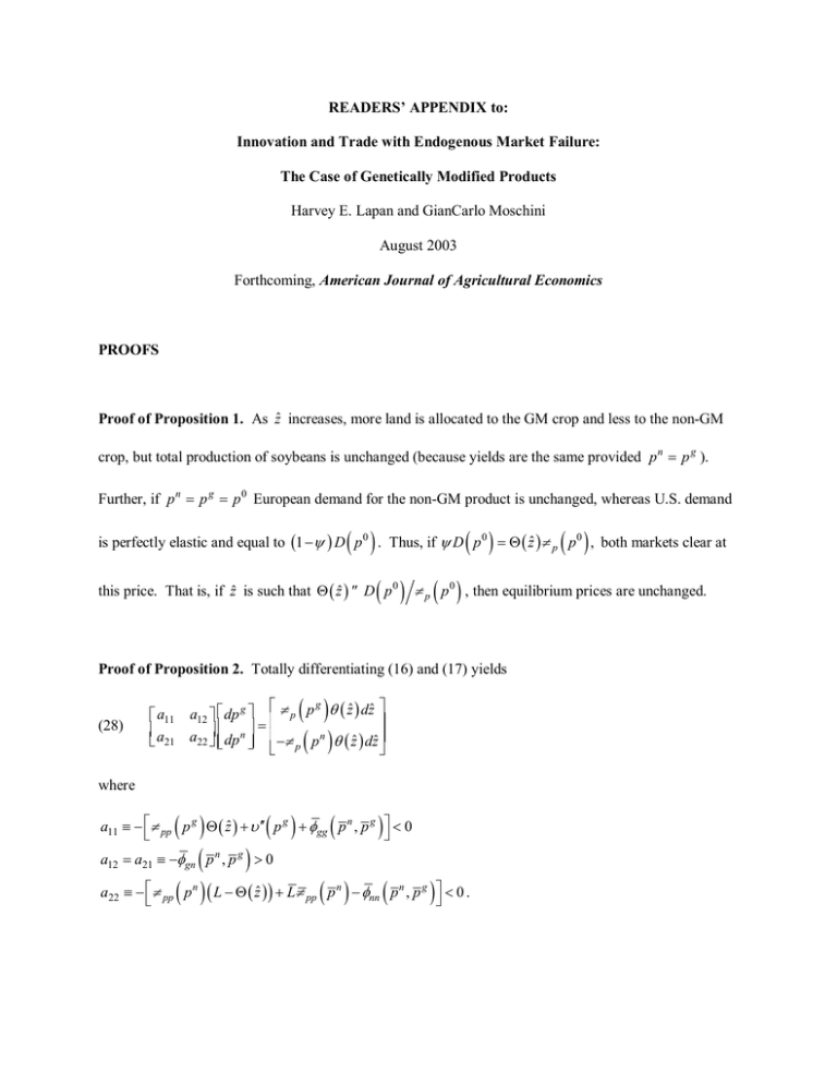
Proof of Proposition 2. Totally differentiating (16) and (17) yields
(28)
a11
a12
dp
g
a21 a22
dp
n
( )
−π ( p ) θ ( zˆ ) dzˆ
π p p g θ ( zˆ ) dzˆ
=
n
p
where
( )
( ) (
) <0
= a ≡ −φ ( p , p ) > 0
≡ − π ( p ) ( L − Θ ( zˆ ) ) + Lπ ( p ) − φ ( p , p )
a11 ≡ − π pp p g Θ ( zˆ ) + υ ′′ p g + φgg p n , p g
a12
n
21
g
gn
a22
n
pp
n
pp
n
nn
g
< 0.
The signs for a11 and a22 come from the convexity of the profit and indirect utility functions whereas the
sign for a12 = a21 comes from the final goods being substitutes in consumption. Because p g < p n ,
realized yields per acre will be higher on non-GM lands. Solving (28) yields
( )
−π ( p ) θ ( zˆ ) dzˆ
π p p g θ ( zˆ ) dzˆ
dp
(29)
g
dp n
= (1 ∆ )
a22
− a12
− a21
a11
n
p
( )
( )
where ∆ = ( a11a22 − a12 a21 ) > 0 . Because p g < p n for ẑ > z 0 , then π p p n > π p p g (i.e., yields are
positively affected by output price provided π pp > 0 ). Thus, given price, total output declines as land
(
(
)
( )) .
( )
planted with the GM crop expands. From (29), dp n dzˆ = (θ ( zˆ ) ∆ ) − a11π p p n − a21π p p g
( )
( )
Because p n ≥ p g , then π p p n ≥ π p p g . Further, a11 < 0 , and, by the assumed Condition 1,
( a11 + a12 ) < 0,
provided that π pp > 0 or υ ′′ > 0 . Thus:
( −a π ( p ) − a π ( p )) > −π ( p ) ( a
n
g
11 p
( dp
) (
11
p
) = ( −θ ( zˆ ) ∆ ) (( a
dzˆ − dp g dzˆ
n
g
21 p
11
(
)
+ a21 ) > 0 , proving dp n dzˆ > 0 . And, from (29)
( )) . Given convexity,
( )
+ a12 ) π p p n + ( a22 + a21 ) π p p g
(
) (
)
Condition 1 guarantees ( a11 + a12 ) < 0 and ( a21 + a22 ) < 0 , proving dp n dzˆ > dp g dzˆ .
(
) (
)
As for part (iii) of Proposition 2, Europe’s welfare can be written as W = Lπ p n ( zˆ ) + φ p n ( zˆ ) , p g ( zˆ ) .
( dW
Thus,
(
)
dzˆ ) = Lπ p p n ( zˆ ) + φn
( dp
n
)
(
dzˆ + φg dp g dzˆ
) ={ S
n
− Dn
( dp
n
)
(
where D n − S n is imports of the non-GM product and D g is imports of the GM product. From
(
)
(
) (
)
Proposition 2, dp n dzˆ > 0 and dp n dzˆ > dp g dzˆ ; thus, for D n − S n > D g ≥ 0 , the result is
proven.
2
)}
dzˆ − D g dp g dzˆ ,
Proof of Proposition 3. From the solution to (19)-(21), and recalling (8)-(10), we have
(
( dp
)
dc ) =
( )
( p ) + υ ′′ ( p ) + φ
dp b dc = − Lπ pp p f + φ ff + φbf
(30)
f
Lπ pp
b
b
bf
( )
∆
( )
+ φbb
∆
( )
(
where ∆ ≡ Lπ pp p b + Lπ pp p f + υ ′′ p b + φ ff + 2φbf + φbb
and φij ≡ ∂ 2φ p f , p b
)
∂pi ∂p j ,
i, j ∈ { f , b} . Convexity of the profit and indirect utility functions guarantees that ∆ is positive (the
excess supply function is positively sloped). If Europe does not consume the GM variety, the numerator
of the first line in (30) is negative, whereas that of the second is positive. But if Europe does consume the
GM product we cannot unambiguously sign both numerators (one must be positive). However, under the
assumed Condition 1, the numerator of the first line must be negative, and that of the second positive.
Proof of Lemma 1. See text.
Proof of Proposition 4. We have shown previously that dp b dc < 0 . The changes in home, foreign, and
hence world welfare are
( ) ( )(
)
(
)
( dW dc ) = Lπ ( p ) + φ ( p , p ) ( dp dc ) + φ ( p , p ) ( dp dc ) =
( d (W + W ) dc ) = Lπ ( p ) + φ ( p , p ) = S − D < 0 .
( dW
dc ) = Lπ p p g + υ ′ p b
dp b dc = S n + S g − D dp b dc < 0
f
f
p
b
f
f
f
b
b
given: pb = p g = p n
b
S n − Dn
( dp
f
)
(
dc − D g dp b dc
f
p
f
b
n
n
f
U.S. welfare declines because it is a net exporter, and the farmgate price declines. World welfare declines
because of the increased verification costs. Europe’s welfare is reduced by the effective cost increase for
imports of the GM-free product (including verification costs), but Europe may benefit from the reduced
price of the GM product, so that the overall impact is ambiguous. Around c = 0 , all parties are hurt.
Proof of Proposition 5. Part (i) follows from the previous section and the immediately preceding
discussion where we have shown that, given ẑ ≤ z 0 , (a) if c=0, then prices are independent of z; whereas
3
)
(
)
(b) given zˆ ∈ 0, z 0 , p b is a declining function of c, while p f is an increasing function of c. Part (ii)
follows from the fact that the introduction of the GM product leads to a decline in the U.S. terms of trade.
The welfare gain to the United States due to the introduction of GM seeds is ∆W =
zˆ
0
η ( z )θ ( z ) dz ,
whereas the welfare loss in the United States depends upon the magnitude of the decline in the terms of
trade. If verification costs are small, then the gains will outweigh the losses; however, for large enough
verification costs the introduction of GM product may lower U.S. welfare.
Proof of Proposition 6. Totally differentiating yields the following comparative statics effects:
(
( dp
)
dt ) =
dp b dt = − φ fb + φbb
(31)
b
∆
( )
( )
Lπ pp p b + Lπ pp + υ ′′ p b + φ ff + φ fb
( )
( )
( )
∆
where ∆ ≡ Lπ pp p b + Lπ pp p f + υ ′′ p b + φ ff + 2φbf + φbb
(
φij ≡ ∂ 2φ p f , p b
( dp
f
) (
)
and
∂pi ∂p j , (i, j ) ∈ { f , b} . Given the identity of U.S. prices for the two varieties,
)
(
)
(
)
dt = dp b dt . Under the assumption of Condition 1, we have dp b dt > 0 > dp b dt . This
establishes the proof of parts (i) and (ii). The proof of (iii) follows from
( dW dt ) = ( Lπ p + φ f ) ( dp f
)
(
) (
dt + (φb ) dp b dt = S n − D f
)( dp
f
)
(
)
dt − D b dp b dt .
The first expression is the welfare gain due to the improved terms of trade on GM-free product imports
(U.S. prices decline), whereas the second term measures the loss due to the worsened gross terms of trade
on the GM product. Note that these costs operate like a tariff on the GM product, assuming the tariff
revenue is thrown away. Clearly, if GM-free imports are large enough, or if imports of the GM product
are low enough, the expression will be positive. Further, as t increases, net imports of GM-free goods
will increase; those of the GM product will decrease, so the expression is even more likely to be positive.
4
Proof of Lemma 2. Totally differentiating (22)-(23) and rearranging yields
dp n
(32)
1
=
∆
dp g
a22
− a12
−a21
a11
bn
bg
where
( ( ) ( L − Θ ( zˆ ) ) + Lπ ( p ) + φ ( p
a11 = π pp p n
n
pp
f
ff
(
)
= (π ( p ) Θ ( zˆ ) + υ ′′ ( p ) + φ ( p
, pb
)) > 0
a12 = a21 = φ fb p n , p g < 0
g
a22
g
pp
bb
(
)
2
∆ = a11a22 − a12
>0
{
f
, pb
)) > 0
( )
( ) (
= − {θ ( zˆ ) π ( p ) dzˆ + a dc + φ dt} .
bn = θ ( zˆ ) π p p n dzˆ − Lπ pp p n + φ ff p f , p b
bg
) dc − a dt}
12
g
p
12
bb
{
)
From (32) the following comparative statics are readily derived:
(33)
(
( ∂p
g
)
( )
(
( )
( )
∂zˆ ) = ( −θ ( zˆ ) ∆ ) { π ( p ) ( L − Θ ( zˆ ) ) + Lπ ( p ) π ( p ) + φ
∂p n ∂zˆ = (θ ( zˆ ) ∆ ) π pp p g Θ ( zˆ ) + υ ′′ p g
(
n
n
pp
(
π p p n + φbbπ p p n + φbf π p p g
pp
g
p
( )
) }
>0
(
g
+ φbf π p p n
ff π p p
)
where the sign of ∂p n ∂zˆ is determined with the help of Condition 1 [i.e., (φbb + φbf ) > 0 ]. Again,
( ∂p
g
)
(
)
∂zˆ cannot be unambiguously signed, except around p g = p n , in which case φ ff + φ fb > 0
(
)
(
)
suffices to imply ∂p g ∂zˆ <0. However, regardless of the sign of ∂p g ∂zˆ , it must be true that
( ∂p
n
) (
)
∂zˆ > ∂p g ∂zˆ , provided that the demand assumption holds.
Similarly, holding ẑ constant, comparative statics for changes in c and t are
(34)
( ∂p
( ∂p
( ∂p
n
f
)
{ ( ( ) ) }
∂c ) = (1 ∆ ){a π ( p ) ( L − Θ ( zˆ ) )} > 0
∂c ) = ( ∂p ∂c ) = ( −a ∆ )π ( p ) ( L − Θ ( zˆ ) ) > 0
2
∂c = ( −1 ∆ ) a22 Lπ pp p n + φ ff − a12
<0
n
22 pp
g
b
n
12
pp
5
) }
( ∂p
( ∂p
( ∂p
(35)
n
g
) (
)
∂t ) = ( −1 ∆ ) ( a φ − a ) < 0
∂t ) = (1 + ( ∂p ∂t )) = (1 ∆ ) a
2
12
11 bb
b
{ ( )
( )} > 0 ;
∂t = ∂p f ∂t = ( −1 ∆ ) {a22 a12 − a12φbb } = ( − a12 ∆ ) π pp p g Θ ( zˆ ) + υ ′′ p g
g
11
( )
( )
π pp p g Θ ( zˆ ) + υ ′′ p g
>0.
Proof of Proposition 7. The impact on price and GM acreage for the case when zˆ = z 0 ( c, t ) is readily
demonstrated, using (32), by setting p ≡ p n = p g (and hence dp = dp n = dp g ), and by bringing dzˆ to the
) left-hand side of the equation. Doing so, and inverting, yields
dp
(36)
dz 0
1
=
∆′
θ ( zˆ ) π p ( p ) θ ( zˆ ) π p ( p ) h p
− ( a22 + a12 )
where
( a11 + a12
∆′ ≡ θ ( zˆ ) π p ( p )( a11 + a22 + 2a12 ) > 0
{
( )
(
h p = − Lπ pp p n + φ ff p f , p b
)
dc + a12dt
hzˆ = − {a12 dc + φbb dt}
hzˆ
}
and where aij are as defined in the proof of Lemma 2. Proceeding as earlier, using the same demand
assumptions, it is readily verified that
(37)
( dp ( c, t ) dc ) ∈ ( −1,0 )
( dp ( c, t ) dt ) ∈ ( −1,0 )
and
( dz
( dz
0
0
)
( c, t ) dt ) < 0
( c, t )
dc > 0
where p n = p g = p, whereas European prices are such that p f = ( p + c ) and p b = ( p + t ) . What
remains to be shown is the impact of higher t on monopoly profits. The result follows because, given the
(
corner solution, d Π M dt
)
z 0 ( c ,t ), p n = p g
(
(
= d Π M dzˆ
by virtue of the corner solution, d Π M dzˆ
)
z0
) ( dz
z0
0
( c, t )
)
dt < 0 , where the sign follows because,
(
)
> 0, and we have shown that dz 0 ( c, t ) dt < 0 .
6