Product Variety and the Gains from International Trade
Feenstra, Robert C.
University of California, Davis
Introduction:
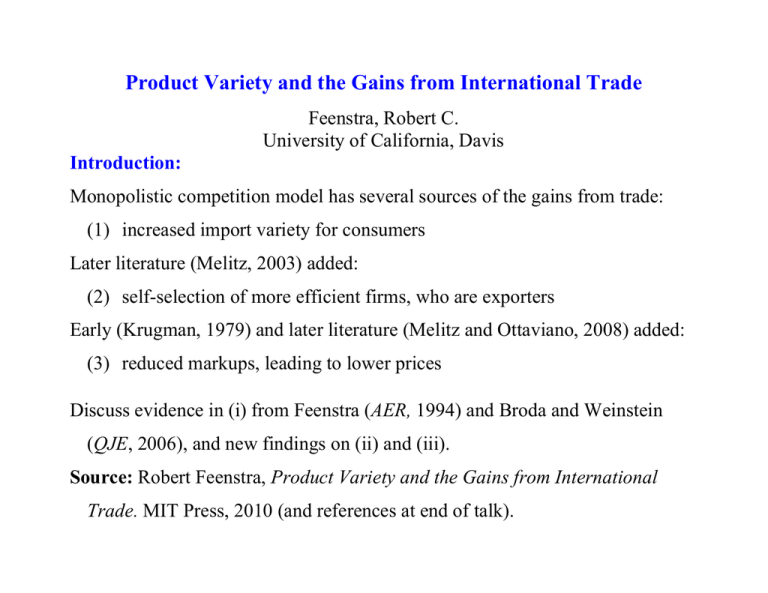
Monopolistic competition model has several sources of the gains from trade:
(1) increased import variety for consumers
Later literature (Melitz, 2003) added:
(2) self-selection of more efficient firms, who are exporters
Early (Krugman, 1979) and later literature (Melitz and Ottaviano, 2008) added:
(3) reduced markups, leading to lower prices
Discuss evidence in (i) from Feenstra (AER, 1994) and Broda and Weinstein
(QJE, 2006), and new findings on (ii) and (iii).
Source: Robert Feenstra, Product Variety and the Gains from International
Trade. MIT Press, 2010 (and references at end of talk).
2
1. Consumer Gains due to Product Variety:
Treat the price of a new good as its reservation price, where demand is zero. For
CES case with >1, reservation price is infinite. But we still get a bounded
region of consumer gain:
p
A
Integrating demand curve with constantelasticity  above the price shows that:
A
1

B (   1)
B
q
3
Feenstra, AER, 1994: Generalize this to many new goods -
Work with the non-symmetric CES function,

(  1) /  
U t  U (q t , I t )    a it q it

i

I
 t

 /(  1)
,   1,
where ait > 0 are parameters and It denotes the set of goods available in period t,
at the prices pit. The CES unit-expenditure function dual to this is,


e( p t , I t )    b it p1it  
iI t

1 /(1  )
,   1, b it  a it .
First consider the case where It-1 = It = I, and bit-1 = bit. Assume that qit are
optimal for the prices and utility, that is, q it  U t (e / pit ) . Then:
4
Theorem 1 (Sato, 1976; Vartia, 1976)
If the set of goods available is fixed at It-1 = It = I, and the parameters bit-1 = bit
are constant, then the ratio of unit-expenditure can be measured by the index:
 p 
e( p t , I )
 PSV ( p t 1 , p t , q t 1 , q t , I )    it 
e ( p t 1 , I )
iI  p it 1 
where w i ( I ) are constructed from the shares sit(I)  p it q it
 s it ( I ) – s it 1 ( I ) 

w i ( I )  
 ln s it ( I ) – ln s it 1 ( I ) 
wi ( I )
,
iI p it q it as,
 s it ( I ) – s it 1 ( I ) 
 .
 
iI  ln s it ( I ) – ln s it 1 ( I ) 
The “Sato-Vartia” weights w i ( I ) are logarithmic means of sit and sit-1,
normalized to sum to unity.
5
Now consider the case where the set of goods is changing over time, but
I t 1  I t   . We again let e(p,I) denote the unit-expenditure function defined
over the goods within the set I. Then the ratio e(pt,I)/e(pt-1,I) is still measured by
the Sato-Vartia index. Our interest is in the ratio e(pt,It)/e(pt-1,It-1), which can be
measured as follows:
Theorem 2 (Feenstra, 1994)
Assume that bit-1 = bit for i  I  I t 1  I t   . Then for  > 1:
  ( I) 
e( p t , I t )

 PSV ( p t 1 , p t , q t 1 , q t , I ) t
e ( p t 1 , I t 1 )
  t 1 ( I ) 
where values t(I) and t-1(I) are constructed as:
1 /(  1)
,
6
  iI p i q i 
  iI ,iI p i q i 



 ,  = t-1,t.
  ( I) 
 1 


 

p
q
p
q
i
i
i
i




i
I
i
I








Each of the terms (I) < 1 can be interpreted as the period  expenditure on
the goods in the set I, relative to the period  total expenditure. Alternatively,
this can be interpreted as one minus the period  expenditure on “new” goods
(not in the set I), relative to the period  total expenditure.
 t ( I )1 /(  1) is the reduction in expenditure due to new product varieties.
 t 1 ( I )1 /(  1) is the increase in expenditure due to disappearing varieties.
See this in a graph:
7
Move from having just good one available (A), to both goods (C):
q2t
D
B
C
A
q1t
With only q1 is available at A, the cost of achieving U is the budget line AB
With q1 and q2 available, the cost of achieving U is the budget line through C
Inward shift in the budget line measures consumer gain from product variety.
8
Applications:
a) New method to estimate the “Armington” elasticity of substitution
between varieties of a good available from different source countries
(Feenstra, AER, 1994):
 Conventional estimates of this elasticity suffer from downward bias due to
simultaneous equation bias and measurement error in unit-values
 New method can be developed that exploits the panel nature of the dataset
(multiple countries over multiple years), and relies on heteroskedasticity in
the errors across countries
 This is “identification through heteroskedasticity” or GMM estimator
 Applied this to six products (men’s leather athletic shoes; men’s and boy’s cotton
knit shirts; stainless/carbon steel bars; color TV; portable typewriters) and obtained
elasticities between 3 and 8; for gold and silver bullion, get 27 or 43.
9
b) U.S. Gains from Import Variety, Broda and Weinstein (QJE, 2006)
Measure the gains to the United States from increased import variety, 1972-2001
U.S. disaggregate imports:
TSUSA (8-digit), 1972-1988
HS (10-digit), 1990-2001
A good is a TSUSA (8-digit) or HS (10-digit), or more aggregate if needed.
A variety is the import to the United States from a source country, like the
“Armington assumption”
 I = set of varieties selling to U.S. in year t and the base year (1972 or 1990),
so that lambda’s are measured as the expenditure on imported varieties from
all other countries relative to the base year.
 Estimated 10,000+ elasticities , with median of 3.7 across HS goods
10
Conclusions:
 There has been large growth in the variety of imported products to the U.S.
 A simple “count” of products should not be used to assess this growth
 The “lambda ratio” is easily constructed from disaggregate trade data, and
allows for a measure of variety growth that is consistent with CES
 The cumulative growth in varieties over 1972-2001 leads to a fall in the
true import price index of 28% by 2001
 That fall in import prices corresponds to gains to the U.S. from
increased import variety which are 2.6% of GDP in 2001
Look at other applications:
 Predicted and actual effects of NAFTA on Mexican exports to the U.S.
(Feenstra and Rose, 1993; Feenstra and Kee, World Economy, 2007)
11
Feenstra and Rose (1993):
 Argued that gains to California from NAFTA will depend on the extent to
which increased agricultural imports/exports change water use
 Estimated the increase in imports of vegetable crops, and their elasticities of
substitution , using GMM methodology
 Social gains from the increase in vegetable imports  $11 million, but social
gains due to reduced water use  $20 million
 did not consider increased exports of water-intensive crops (rice, dairy)
Feenstra and Kee (World Economy, 2007):
 Estimated the “lambda ratio” for goods shipped from Mexico to the
United States, including agricultural goods, during the opening of
NAFTA. This is also called the “extensive margin of trade”:
12
Table 1: Mexico’s Trade with the U.S., 1990-2001
(a) Mexico’s Export Variety to the U.S.
Textiles & Wood Petroleum Mining Machinery
Average Agriculture Garments &Paper & Plastics &Metals &Transport Electronics
1990
51.3
41.5
71.2
47.3
55.4
46.6
65.6
39.5
2001
69.6
50.9
82.6
63.2
72.7
56.4
75.8
65.6
Growth
2.8
1.9
1.4
2.6
2.5
1.7
1.3
4.6
(b) U.S. Tariffs on Imports from Mexico
Textiles & Wood Petroleum Mining Machinery
Average Agriculture Garments &Paper & Plastics &Metals &Transport Electronics
1990
3.2
4.4
13.0
2.2
0.6
2.1
2.5
4.1
2001
0.2
0.8
0.4
0.0
0.1
0.7
0.1
0.1
13
2. Producer Benefits from Export/Output Variety
A. First rationale: When   0 we will denote its positive value by    ,
and using labor resources Lt to replace utility Ut:


L t    a it q (it1) /  

 iI t
 /(  1)
, a it  0,   0.
The maximum revenue obtained using one unit of labor resources is then:
1/( 1)


1
r(p t , I t )   bit pit 
 iIt

,
bit  a it ,   0.
With this reinterpretation, Theorem 2 continues to hold as:
  ( I) 
r(p t , I t )
 PSV ( p t 1 , p t , q t 1 , q t , I ) t

r(p t 1 , I t 1 )
  t 1 ( I ) 
1 /(  1)
,
14
where the exponent appearing on (t/t-1) is now negative. In other words, the
appearance of “new outputs,” so that t < 1, will raise revenue on the producer
side of the economy.
q2t
B
C
q1t
A
If only q1t is available, the economy produces at A, with output revenue AB.
Then if variety 2 becomes available, then economy is at C, with an increase in
revenue. This illustrates the benefits of export/output variety.
15
Problem: if factor proportions between the two varieties are the same, then the
transformation curve is linear, and there is no gain to export/output variety
B. Second Rationale
Can show that in the Melitz (2003) model, there is a concave tradeoff between
export and domestic varieties, even with the same factor intensities!
~
M xt
B
C
A
~
Mt
Gains to export variety depend on the elasticity of transformation .
16
Application: Gains from Export Variety, Feenstra and Kee (JIE, 2008)
 For sample of 48 countries exporting to the U.S. over 1980–2000, find that
average export variety to the United States increases by 3.3% per year, so it
nearly doubles over these two decades.
 That total increase in export variety is associated with a cumulative 3.3%
productivity improvement for exporting countries, i.e. after two decades,
GDP is 3.3% higher than otherwise due to growth in export variety
 That estimate is greater than the welfare gains for the U.S. found by Broda
and Weinstein (2006), which was that after 30 years, real GDP was 2.6%
higher than otherwise due to growth in import variety.
 Export variety is correlated with times series changes in country
productivity, but does not explain that much of cross-section differences
17
 These estimates depend on the elasticity of transformation , which in turn
depends on the elasticity of substitution  and most crucially on , which is
the parameter of the Pareto distribution of firms productivities.
 New results from Arkolakis, Costinot and Rodriguez-Clare (2008, 2009)
argue that the Pareto parameter  and the share of trade are all we need to
know for the gains from trade:
Theorem 2 (Arkolakis, et al, 2008, 2009; Feenstra, CJE, 2010)
The gains from trade in the Melitz (2003) model are:
1

 R dt
w t / PtH

  t where  t  
H
w t 1 / Pt 1
 R dt  R xt

.

So the gains from trade only depend on what a country buys from itself!
18
3. Markups with Translog Preferences
Perhaps the CES case overstates the consumer gains from variety, because the
reservation price is infinite.
p
A
Integrating demand curve with constantelasticity  above the price shows that:
A
1

B (   1)
B
q
Can we develop the analogous theory for other preferences, like translog?
19
Yes! Furthermore, while we will find that the gains from variety are indeed
lower with translog, there is a new source of gains from trade that does not
arise in the CES case: rising imports will have a pro-competitive impact on
reducing U.S. prices and those from all other selling countries, due to reduced
markups. (In contrast, markups are fixed in the CES case).
We find that the pro-competitive gains exceed the import variety gains.
Technical issues with translog:
1. Need to solve for reservation prices for goods not available.
2. To get the right markups, need to allow multiple exporters in each country.
Sufficient to have the Herfindahl indexes of exports from each country,
which we purchased from piers.com and from Statistics Canada.
20
~
Translog unit-expenditure function over the universe of goods N :
~
N
ln e   0   i ln p i  2
1
i 1
~ ~
N N
   ij ln pi ln p j , with ij = ij .
i  1 j 1
To ensure that the expenditure function is homogenous of degree one, we need:
~
N
 i  1, and
i 1
~
N
  ij  0 .
i 1
We will further assume that all goods are “symmetrically” in the ij coefficients:
~

 N  1
~
 ii     ~ , and  ij  ~ for i  j, with i, j = 1,…, N .
N
 N 
~
N
The share equations are:
s i  i    ij ln p j .
j 1
21
~
Suppose si > 0 for i=1,…,N, while sj = 0 for j=N+1,…, N . The we use sj = 0 for
~
p , j=N+1,…, N . These
unavailable goods to solve for the reservation prices ~
j
reservation prices
~
pj
are substituted back into the expenditure function to obtain:
Theorem 3 (Bergin and Feenstra, 2008)
N
ln e  a 0   a i ln p i 
i 1
1
2
N N
  bij ln pi ln p j ,
i 1 j  1
where: b ii    ( N  1) / N, and b ij   / N for i  j with i, j = 1,…,N,


a i  i  N1 1  iN1 i , for i = 1,…,N,


2
 1   N~
 1  N~
2
a 0  0    i  N 1 i    i  N 1 i .
N

 2 
22
~
Now distinguish t-1 and t, with i=N+1,…, N are not available in either period.
The goods {1,…,N} are divided into two (overlapping) sets each period:
 the set i  I  is available in period  = t-1,t, with union I t 1  I t  {1,..., N} ;
 We shall let I  I t 1  I t   denote any non-empty subset of intersection,
with N  0 goods within the set I .
In general, the Törnqvist price index is exact for the translog function:
 et  N 1
ln
   2 (s it  s it 1 )(ln p it  ln p it 1 ).
 e t  1  i 1
Solving for the reservation prices for new and disappearing goods, we obtain the
following expression for the exact price index:
23
Theorem 4 (Feenstra and Weinstein, 2009)
 e 
ln t   
 e t 1  iI
1
(s
2 it
 sit 1 )(ln p it  ln p it 1 )  V,
2
2 



1
1




 


2
2
where, V       s it  s it 1      s it     s it 1   ,
 N   iI   iI
 2    iI
  


and the shares sit 1 and s it are defined as:


si  s i  N1 1   s i  , for i  I , and  = t-1, t.
 iI 
 V is the variety effect. We need to further breakdown prices into marginal
costs and markups, to identify a pro-competitive effect.
24
Optimal Prices:
The optimal price can be written as the familiar markup over marginal costs:
  (p , E ) 
pit  Ci ' [ x i ( p t , E t )]  i t t  .
 i ( p t , E t )  1
The elasticity of demand for the “symmetric” translog is:
it  1 
 ( N t  1)
.
s it N t
It follows that the optimal prices are:

s N 
ln pit  ln C'it  ln 1  it t  ,
  ( N t  1) 
Substitute into the Törnqvist price index to obtain the pro-competitive effect.
25
Problem:
We do not observe firm-level shares. So aggregate prices from the firm to the
country level using Herfindahl indexes:

H it sit N t 
ln pit  ln ln C'it  ln 1 
,

  (N t  1) 
using the Herfindahl index for firm exports by country i, H it   jJ (s ijt ) 2 .
it
 We see that the impact of import competition on prices will depend on the
product H it sit for importing countries i, and also for the United States
 H it sit is interpreted as the “per firm” market shares, where lower market
shares lead to lower markups.
26
Conclusions:
 Fall in market share for many U.S. industries, and a smaller rise in the U.S.
Herfindahls  U.S. firm market shares are falling, along with markups.
 Markups for exporters are lower than U.S. markups, and with rising shares
 a fall in average markup in the U.S. market due to import competition
 There has also been a growth in market share of “new” suppliers, with
corresponding partial variety gains
 Estimates of the sum of the partial variety gains and pro-competitive
impact give a number that is similar to the gains from Broda and
Weinstein (2006), i.e. around 2.6% of GDP in 2001, with 2/3 from procompetitive effect and 1/3 from variety effect.
27
References
Arkolakis, Costas, Svetlana Demidova, Peter J. Klenow, and Andrés Rodríguez-Clare, 2008,
“Endogenous Variety and the Gains from Trade,” American Economic Review, 2008, 444-450.
Arkolakis, Costas, Arnaud Costinot and Andrés Rodríguez-Clare, 2009, “New Trade Model, Same
Old Gains?,” NBER working paper no. 15628.
Bergin, Paul R. and Robert C. Feenstra, 2009, “Pass-through of Exchange Rates and Competition
Between Fixers and Floaters,” Journal of Money, Credit and Banking, February, 41(s1), 35-70.
Feenstra, Robert C. and Andrew K. Rose, 1993, “Trade With Mexico and Water Use in California
Agriculture,” in Peter Garber, The Mexico-U.S. Free Trade Agreement, MIT Press, 189-218.
Feenstra, Robert C. and Andrew K. Rose, 1993, “California Agriculture and an Emerging Mexico,”
North American Journal of Economics and Finance, 4(1), 91-108.
Feenstra, Robert C., 1994, “New Product Varieties and the Measurement of International Prices,”
American Economic Review, 84(1), March, 157-177.
Feenstra, Robert C. and Hiau Looi Kee, 2007, “Trade Liberalization and Export Variety: A
Comparison of Mexico and China,” World Economy, January, 5-22.
Feenstra, Robert C. and Hiau Looi Kee, 2008, “Export Variety and Country Productivity:
Estimating the Monopolistic Competition Model with Endogenous Productivity,” Journal of
International Economics, 74(2), 500-518.
28
Feenstra, Robert C., 2010, “Measuring the Gains from Trade under Monopolistic Competition,”
Canadian Journal of Economics, February, 1-28.
Feenstra, Robert C., 2010, Product Variety and the Gains from International Trade. MIT Press.
Feenstra, Robert C. and David Weinstein, 2010, “Globalization, Competition, and the U.S. Price
Level,” NBER Working Paper no. 15749.
Krugman, Paul R., 1979, ‘Increasing Returns, Monopolistic Competition and International Trade,’
Journal of International Economics, 9, 469-479
Melitz, Marc J., 2003, ‘The Impact of Trade on Intra-Industry Reallocations and Aggregate Industry
Productivity,’ Econometrica, 71(6),1695-1725
Melitz, Marc J. and Giancarlo I. P. Ottaviano, 2008, ‘Market Size, Trade, and Productivity,’ Review
of Economic Studies, 75(1), 295-316
Sato, Kazuo, 1976, ‘The Ideal Log-Change Index Number,’ Review of Economics and Statistics 58,
May, 223-228
Vartia, Y.O., 1976, ‘Ideal Log-Change Index Numbers’, Scandinavian Journal of Statistics 3, 121126