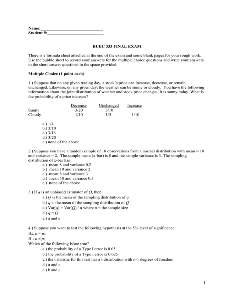
Name:_____________________________
Student #:__________________________
BUEC 333 FINAL EXAM
There is a formula sheet attached at the end of the exam and some blank pages for your rough work.
Use the bubble sheet to record your answers for the multiple choice questions and write your answers
to the short answer questions in the space provided.
Multiple Choice (1 point each)
1.) Suppose that on any given trading day, a stock’s price can increase, decrease, or remain
unchanged. Likewise, on any given day, the weather can be sunny or cloudy. You have the following
information about the joint distribution of weather and stock price changes. It is sunny today. What is
the probability of a price increase?
Sunny
Cloudy
Decrease
3/20
1/10
Unchanged
3/10
1/5
Increase
1/10
a.) 1/4
b.) 3/10
c.) 3/16
d.) 3/20
e.) none of the above
2.) Suppose you have a random sample of 10 observations from a normal distribution with mean = 10
and variance = 2. The sample mean (x-bar) is 8 and the sample variance is 3. The sampling
distribution of x-bar has
a.) mean 8 and variance 0.2
b.) mean 10 and variance 2
c.) mean 8 and variance 3
d.) mean 10 and variance 0.3
e.) none of the above
3.) If q is an unbiased estimator of Q, then:
a.) Q is the mean of the sampling distribution of q
b.) q is the mean of the sampling distribution of Q
c.) Var[q] = Var[Q] / n where n = the sample size
d.) q = Q
e.) a and c
4.) Suppose you want to test the following hypothesis at the 5% level of significance:
H0: μ = μ0
H1: μ ≠ μ0
Which of the following is/are true?
a.) the probability of a Type I error is 0.05
b.) the probability of a Type I error is 0.025
c.) the t statistic for this test has a t distribution with n-1 degrees of freedom
d.) a and c
e.) b and c
1
5.) The significance level of a test is the probability that you:
a.) reject the null when it is true
b.) fail to reject the null when it is false
c.) reject the null when it is false
d.) fail to reject the null when it is true
e.) none of the above
6.) Suppose that Yi = α + βXi + εi and εi = ui + vi + Xi. Assume that u, v, and X are independently
distributed as standard normals. In this case, the OLS estimator, beta-hat, is:
a.) unbiased and efficient
b.) unbiased and not efficient
c.) biased and efficient
d.) biased and not efficient
e.) none of the above
7.) For a model to be correctly specified under the CLRM, it must:
a.) be linear in the coefficients
b.) include all relevant independent variables and their associated transformations
c.) have an additive error term
d.) all of the above
e.) none of the above
8.) The Gauss-Markov Theorem says that when the 6 classical assumptions are satisfied:
a.) The least squares estimator is unbiased
b.) The least squares estimator has the smallest variance of all linear estimators
c.) The least squares estimator has an approximately normal sampling distribution
d.) The least squares estimator is consistent
e.) None of the above
9.) The OLS estimator is said to be unbiased when:
a.) Assumptions 1 through 2 are satisfied
b.) Assumptions 1 through 3 are satisfied
c.) Assumptions 1 through 4 are satisfied
d.) Assumptions 1 through 5 are satisfied
e.) Assumptions 1 through 6 are satisfied
10.) The sampling variance of the slope coefficient in the regression model with one independent
variable:
a.) will be smaller when there is more variation in ε
b.) will be larger when there is less variation in ε
c.) will be smaller when there is more variation in X
d.) will be larger when there is more co-variation in ε and X
e.) none of the above
11.) Omitting a relevant explanatory variable that is uncorrelated with the other independent variables
causes:
a.) bias and no change in variance
b.) bias and an increase in variance
c.) bias and a decrease in variance
d.) no bias
e.) none of the above
2
12.) Consider that the correct model is Yi = α + β1X1i + β2X2i + εi. Instead, you base your OLS
estimates on the following model where Yi = α + β1X1i + εi. The correlation between X1i and X2i is
positive. Furthermore, the population regression coefficient β2 is positive. The bias for the OLS
estimator of β1:
a.) is positive
b.) is negative
c.) is zero
d.) cannot be determined with the information provided.
e.) none of the above.
13.) In a regression explaining earnings, you include one independent variable: an individuals' number
of years of education as an independent variable but nothing else. You know that more educated
people earn more. You also know that more educated people drink more. In this case, the bias for the
OLS estimate of the effect of education on earnings:
a.) is positive
b.) is negative
c.) is zero
d.) cannot be determined with the information provided.
e.) none of the above.
14.) Suppose we estimate the linear regression Yˆi  10  2 X i  5Di where Yi is person i’s hourly
wage, Xi is years of employment experience, and Di equals one for men and zero for women. If we
define a new variable Fi equal to one for men and zero for women instead, the least squares estimates
would be:
a.) Yˆi  5  2 X i  5Fi
b.) Yˆi  5  2 X i  5Fi
c.) Yˆi  10  2 X i  5Fi
d.) Yˆi  10  2 X i  5Fi
e.) none of the above
15.) Apart from inflating the F statistic and R2, there is another potential problem with excluding the
constant term. By doing so, we are likely to make the OLS estimates of our included independent
variables:
a.) unbiased
b.) inefficient
c.) inconsistent
d.) unstable
e.) none of the above
3
Short Answer (10 points each – show your work!)
1.) An oil exploration firm has recently acquired the drilling rights to two sites, one in Alberta and one
in Texas. The exact quantity of oil that can be extracted from each site is unknown. A geophysicist
estimates that the quantity of oil (in millions of barrels) at Site A is independent of the quantity of oil
at Site B. Based on the available evidence, he assigns the following probability distribution to the
quantities that can be extracted from each site:
Site A quantity
Probability
0
1/4
1
1/2
2
1/4
Site B quantity
Probability
0
1/6
1
1/2
2
1/3
a.) What is the probability that the total quantity of oil that can be extracted from the two sites
is exactly 2 million barrels?
b.) After purchasing the drilling rights, the firm conducts a test drilling at site A. The test drilling
indicates that 1 million barrels can be extracted from that site. What is the expected total
quantity of oil that can be extracted from the two sites?
4
2.) Suppose we have a linear regression model with one independent variable and no intercept:
Yi = βXi + εi
Suppose also that εi satisfies the six classical assumptions.
a.) Verbally, explain the steps necessary to derive the least squares estimator.
b.) Formally, derive a mathematical expression for this estimator given your answer in part a).
5
Page intentionally left blank. Use this space for rough work or the continuation of an answer.
6
3.) Consider the following equation for a sample of divorced men who failed to make at least one
child support payment in the last four years (standard errors in parentheses):
Pi  2.0  0.50M i  25.0Yi  0.80 Ai  3.0 Bi  0.15Ci
(0.10)
(20.0) (1.00) (3.0) (0.05)
Where: P is the number of missed child support payments for the i-th divorced man
Y is the share of income taken up by child support payments for the i-th divorced man
M is the number of months of unemployment for the i-th divorced man
A is the age of the i-th divorced man
B is an index of how strongly the i-th divorced man expresses his religious beliefs
C is the number of children for the i-th divorced man
a.) What is the unit of measurement of a standard error?
b.) Why is the standard error of Y so much larger than that of C? Hint: think of the Venn diagrams
developed in Lecture 12.
c.) You expected that the coefficients on M and Y are positive. Test these two hypotheses at the 5%
level of significance, assuming that N is so large that t converges on a normal distribution.
d.) Test the hypothesis that the coefficient on A is not zero at the 1% level of significance.
e.) Are there any potential violations of the CLRM in the equation above? If so, what are they and
what do they imply about your answers to c) and d) above?
7
Page intentionally left blank. Use this space for rough work or the continuation of an answer.
8
4.) Suppose the data generating process is:
ln(WAGE )  0  1 ( EXPERIENCE)  2 ( EDUCATION)  3 (MALE)  4 ( AGE)  
where: WAGE is the wage earned in the labour market;
EXPERIENCE is number of years of labour market experience;
EDUCATION is years of formal education;
MALE is a dummy variable that equals 1 if a person is male, and 0 otherwise;
AGE is a person’s age.
a.) If you omit EXPERIENCE from the model, how do you expect it to affect your estimate of β4?
Be precise, and explain your reasoning.
b.) What if you omit MALE instead? Be precise, and explain your reasoning.
c.) Now suppose that 1  0 . Does that change your answer to part a? Explain.
d.) Now suppose you want to test whether the marginal effect of AGE is the same for men and for
women. How would you test this hypothesis?
9
Page intentionally left blank. Use this space for rough work or the continuation of an answer.
10
5.) You have been hired by a hedge fund as a market analyst. Your first day on the job, your boss tells
you that oil prices have her “worried about excess portfolio volatility” and that she is “looking for
investments that hedge against future oil price increases”. She asks you to analyze the relationship
between oil prices and the rate of return on several assets, hoping that you can find one asset whose
returns are unrelated to oil prices and one asset whose returns are negatively related to oil prices. You
spend the better part of the day running least squares regressions and settle on this one (standard
errors in parentheses):
ln Oˆ t  3.73  0.00041At  0.025Bt
(0.45) (0.00001) (0.001)
n  43 R 2  0.35 F  10.8 rAB  0.02
where: Ot is the price of one barrel of crude oil in month t
At is the monthly rate of return on shares of Apple of California
Bt is the monthly rate of return on shares of the Potash Corporation of Saskatchewan
rAB is the sample correlation between At and Bt
a.) Interpret the value of the R2 and the F statistic (assume a critical value of 3.23)
b.) Interpret the estimated coefficients on At and Bt.
c.) One of your co-workers thinks Bt satisfies your boss’ request for an asset “whose returns are
negatively related to oil prices”. Another co-worker thinks you should test this to be sure.
State the appropriate null hypothesis, test it, and interpret the result.
d.) One of your co-workers thinks At satisfies your boss’ request for an asset “whose returns are
unrelated to oil prices”. Another co-worker disagrees because “the coefficient on At is
statistically significant”. Which of them is correct? Explain.
11
Page intentionally left blank. Use this space for rough work or the continuation of an answer.
12
6.) The first half of the course was dedicated to developing the least squares estimator. The rest of the
course was dedicated to considering those instances when problems with the least squares estimator
arise. Underlying the discussion, there were the six assumptions of the classical linear model.
a.) Name the six assumptions and explain what each of them mean.
b.) Some of these assumptions are necessary for the OLS estimator to be unbiased. Some of these
assumptions are necessary for the OLS estimator to be “best”. Explain the distinction between
these two concepts.
c.) Indicate which of the six assumptions are necessary for the OLS estimator to be unbiased and
which of the six assumptions are necessary for the OLS estimator to be “best”.
d.) In general, would you prefer your estimates to be biased but efficient or unbiased but not efficient?
Explain your answer.
13
Page intentionally left blank. Use this space for rough work or the continuation of an answer.
14
Useful Formulas:

k

k
Var ( X )  E  X   X    xi   X  pi
E ( X )   pi xi
i 1
k
Pr( X  x)   Pr X  x, Y  yi 
2
i 1
m
E Y | X  x    yi PrY  yi | X  x 
E Y    E Y | X  xi  Pr X  xi 
i 1
k
i 1
Pr( X  x, Y  y)
Pr( X  x)
Pr(Y  y | X  x) 
k
2
i 1
Ea  bX  cY   a  bE( X )  cE (Y )
Var (Y | X  x)    yi  E Y | X  x  PrY  yi | X  x 
2
i 1
Cov( X , Y )   x j   X  yi  Y  PrX  x j , Y  yi 
k
m
i 1 j 1
Cov X , Y 
Var  X Var Y 
Corr  X , Y    XY 
Var aX  bY   a 2Var ( X )  b 2Var (Y )  2abCov( X ,Y )
E Y 2   Var (Y )  E (Y ) 2
Cova  bX  cV ,Y   bCov( X ,Y )  cCov(V ,Y )
E XY   Cov( X ,Y )  E( X ) E(Y )
x
n
1
 xi
n i 1
Var a  bY   b 2Var (Y )
s2 
x
s/ n
1 n

 xi  x  yi  y 
n  1 i 1
t
n
1
xi  x 2

n  1 i 1
s XY
 X
n
For theregression model Yi   0  1 X i   i , ˆ1 
i

 X Yi  Y
βˆ0  Y  ˆ1 X
 X
i
X

2
1
 X
i
i
   e /n  k 
2
2
X
s.e. ˆ1 

2
i i
 X
i
i
X
Z

2
 Y  Y    Yˆ  Y    e
n
i 1
R2
n
2
i
i 1
2
i
n
i 1
 e /( n  k  1)  1  (1  R
 1
 Y  Y  /( n  1)
2
i
F
i
 Yˆ  Y 

 Y  Y 
2
n 1
2
)
n  k 1
ESS / k
R2 / k

RSS /(n  k  1) (1  R 2 ) /(n  k  1)
RSS1  RSS2 / M
F
RSS2 /(n  k  M  1)
2
i i
ˆ j   H
s.e.(ˆ j )
ˆ j   H
Var[ ˆ j ]
Yˆi  ˆ0  ˆ1 X 1i  ˆ2 X 2i    ˆk X ki
2
i
2
i i

 e /n  k 
t
i 1
Var ( ˆ ) 
X 
rXY  s XY / s X sY
s2 

i 1
n
Z
R
2
i
i
i
i
2
e

d

T
t 2
t
 1
e
 Y  Y 
2
i i
2
i
i
 et 1 
2
T
e2
t 1 t
15
16