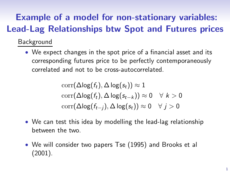
Example of a model for non-stationary variables:
Lead-Lag Relationships btw Spot and Futures prices
Background
• We expect changes in the spot price of a financial asset and its
corresponding futures price to be perfectly contemporaneously
correlated and not to be cross-autocorrelated.
corr(∆log(ft ), ∆ log(st )) ≈ 1
corr(∆log(ft ), ∆ log(st−k )) ≈ 0
∀k>0
corr(∆log(ft−j ), ∆ log(st )) ≈ 0
∀j>0
• We can test this idea by modelling the lead-lag relationship
between the two.
• We will consider two papers Tse (1995) and Brooks et al
(2001).
1
Futures & Spot Data
• Tse (1995): 1055 daily observations on NSA stock index and
stock index futures values from December 1988 - April 1993.
• Brooks et al (2001): 13,035 10-minutely observations on the
FTSE 100 stock index and stock index futures prices for all
trading days in the period June 1996 – 1997.
2
Methodology
• The fair futures price is given by
∗
(r −d)(T −t)
Ft = St e
where Ft∗ is the fair futures price, St is the spot price, r is a
continuously compounded risk-free rate of interest, d is the
continuously compounded yield in terms of dividends derived
from the stock index until the futures contract matures, and
(T − t) is the time to maturity of the futures contract.
Taking logarithms of both sides of equation above gives
∗
ft = st +(r − d)(T − t)
• First, test ft and st for nonstationarity.
3
Dickey-Fuller Tests on Log-Prices and Returns for
High Frequency FTSE Data
Dickey–Fuller statistics
for log-price data
Dickey–Fuller statistics
for returns data
Futures
−0.1329
Spot
−0.7335
−84.9968
−114.1803
• Conclusion: log Ft and log St are not stationary, but ∆ log Ft
and ∆ log St are stationary.
• However, a model containing only first differences has no long
run relationship.
• Solution: see if there exists a cointegrating relationship
between ft and st which would allow us to include levels terms
in this framework.
4
Cointegration test regression and test on resid.
• Potential cointegrating regression:
st = γ0 + γ1 ft + zt
where zt is a disturbance term.
• Estimate the regression, collect the residuals, zˆt , and test
whether they are stationary (using high-freq. FTSE data).
Coefficient
γ̂0
γ̂1
Estimated value
0.1345
0.9834
DF test on residuals
ẑt
Test statistic
−14.7303
Source: Brooks, Rew and Ritson (2001).
• Conclusion: zˆt are stationary and therefore we have a
cointegrating relationship between log Ft and log St .
5
• Final stage in Engle-Granger 2-step method is to use the first
stage residuals, ẑt as the equilibrium correction term in the
general equation.
• The overall model is
∆ log st = β0 + δẑt−1 + β1 ∆ ln st−1 + α1 ∆ ln ft−1 + vt
Coefficient
β̂ 0
δ̂
β̂ 1
α̂1
Estimated value
9.6713E−06
−0.8388
0.1799
0.1312
t-ratio
1.6083
−5.1298
19.2886
20.4946
Source: Brooks, Rew and Ritson (2001).
• α̂1 is positive and highly significant
• β̂ 1 is positive and highly significant
• δ̂ is negative and highly significant
6
Forecasting High Frequency FTSE Returns
• Is it possible to use the error correction model to produce
superior forecasts to other models?
Comparison of Out of Sample Forecasting Accuracy
RMSE
MAE
% Correct direction
ECM
0.0004382
0.4259
67.69%
ECM-COC
0.0004350
0.4255
68.75%
ARIMA
0.0004531
0.4382
64.36%
VAR
0.0004510
0.4378
66.80%
Source: Brooks, Rew and Ritson (2001).
7
Can Profitable Trading Rules be Derived from the
ECM-COC Forecasts?
• The trading strategy involves analysing the forecast for the
spot return, and incorporating the decision dictated by the
trading rules described below. It is assumed that the original
investment is £1000, and if the holding in the stock index is
zero, the investment earns the risk free rate.
– Liquid Trading Strategy - making a round trip trade (i.e. a
purchase and sale of the FTSE100 stocks) every ten minutes
that the return is predicted to be positive by the model.
– Buy-&-Hold while Forecast Positive Strategy - allows the
trader to continue holding the index if the return at the next
predicted investment period is positive.
– Filter Strategy: Better Predicted Return Than Average involves purchasing the index only if the predicted returns are
greater than the average positive return.
8
Can Profitable Trading Rules be Derived from the
ECM-COC Forecasts? (Cont’d)
– Filter Strategy: Better Predicted Return Than First Decile only the returns predicted to be in the top 10% of all returns
are traded on
– Filter Strategy: High Arbitrary Cut Off - An arbitrary filter of
0.0075% is imposed,
9
Spot Trading Strategy Results for Error Correction
Model Incorporating the Cost of Carry
Trading strategy
Passive investment
Terminal
Wealth
(£)
1040.92
Liquid trading
1156.21
Buy-and-Hold while
forecast positive
Filter I
1156.21
1144.51
Filter II
1100.01
Filter III
1019.82
Return(%)
annualised
4.09
{49.08}
15.62
{187.44}
15.62
{187.44}
14.45
{173.40}
10.00
{120.00}
1.98
{23.76}
Terminal
Wealth (£)
with slippage
1040.92
1056.38
1055.77
1123.57
1046.17
1003.23
Return(%)
Annualised
with slippage
4.09
{49.08}
5.64
{67.68}
5.58
{66.96}
12.36
{148.32}
4.62
{55.44}
0.32
{3.84}
Number
of trades
1
583
383
135
65
8
Source: Brooks, Rew and Ritson (2001).
10
Conclusions
• The futures market “leads” the spot market because:
• the stock index is not a single entity, so
• some components of the index are infrequently traded
• it is more expensive to transact in the spot market
• stock market indices are only recalculated every minute
• Spot & futures markets do indeed have a long run
relationship.
• Since it appears impossible to profit from lead/lag
relationships, their existence is entirely consistent with the
absence of arbitrage opportunities and in accordance with
modern definitions of the efficient markets hypothesis.
11