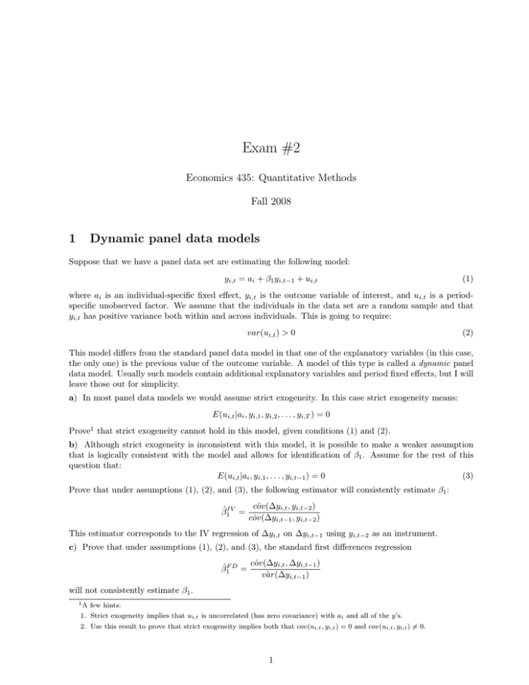
Exam #2
Economics 435: Quantitative Methods
Fall 2008
1
Dynamic panel data models
Suppose that we have a panel data set are estimating the following model:
yi,t = ai + β1 yi,t−1 + ui,t
(1)
where ai is an individual-specific fixed effect, yi,t is the outcome variable of interest, and ui,t is a periodspecific unobserved factor. We assume that the individuals in the data set are a random sample and that
yi,t has positive variance both within and across individuals. This is going to require:
var(ui,t ) > 0
(2)
This model differs from the standard panel data model in that one of the explanatory variables (in this case,
the only one) is the previous value of the outcome variable. A model of this type is called a dynamic panel
data model. Usually such models contain additional explanatory variables and period fixed effects, but I will
leave those out for simplicity.
a) In most panel data models we would assume strict exogeneity. In this case strict exogeneity means:
E(ui,t |ai , yi,1 , yi,2 , . . . , yi,T ) = 0
Prove1 that strict exogeneity cannot hold in this model, given conditions (1) and (2).
b) Although strict exogeneity is inconsistent with this model, it is possible to make a weaker assumption
that is logically consistent with the model and allows for identification of β1 . Assume for the rest of this
question that:
E(ui,t |ai , yi,1 , . . . , yi,t−1 ) = 0
(3)
Prove that under assumptions (1), (2), and (3), the following estimator will consistently estimate β1 :
β̂1IV =
cov(∆y
ˆ
i,t , yi,t−2 )
cov(∆y
ˆ
i,t−1 , yi,t−2 )
This estimator corresponds to the IV regression of ∆yi,t on ∆yi,t−1 using yi,t−2 as an instrument.
c) Prove that under assumptions (1), (2), and (3), the standard first differences regression
β̂1F D =
cov(∆y
ˆ
i,t , ∆yi,t−1 )
var(∆y
ˆ
i,t−1 )
will not consistently estimate β1 .
1A
few hints:
1. Strict exogeneity implies that ui,t is uncorrelated (has zero covariance) with ai and all of the y’s.
2. Use this result to prove that strict exogeneity implies both that cov(ui,t , yi,t ) = 0 and cov(ui,t , yi,t ) 6= 0.
1
ECON 435, Fall 2008
2
2
Instrumental variables and local average treatment effects
Suppose we are using a scholarship experiment to measure the effect of university attendance on wages.
We have a random sample on (y, p, z) where: zi = I(received scholarship), pi = I(attended university), and
yi is subsequent wages.
Let pi (z) and yi (p) be the potential outcome functions for university attendance and wages2 respectively.
The scholarship is assigned by a random mechanism:
Pr(zi = 1|pi (0), pi (1), yi (0), yi (1)) = Pr(zi = 1) = q
The choice of whether to attend university is not random. Each individual falls into one of four categories:
1. “Always-takers” go to university whether or not they receive the scholarship, i.e., pi (0) = pi (1) = 1.
2. “Never-takers” never go to university, i.e., pi (0) = pi (1) = 0.
3. “Compliers” go to university only if they receive the scholarship, i.e., pi (0) = 0, pi (1) = 1.
4. “Defiers” go to university only if they don’t receive the scholarship pi (0) = 1, pi (1) = 0.
We assume that no one is a defier, i.e., that Pr(def ier) = 0.
We are interested in the treatment effect of university attendance on wages, i.e.:
T Ei = yi (1) − yi (0)
a) Which of the following quantities can be identified in the data?
1. E(p|z = 1) and E(p|z = 0)
2. E(y|z = 1) and E(y|z = 0).
3. E(y|p = 1) and E(y|p = 0).
b) Find Pr(complier) in terms of those quantities listed in part (a) that can be identified in the data.
c) Prove that
E(y|z = 1) − E(y|z = 0)
E(p|z = 1) − E(p|z = 0)
This quantity is known as the “local average treatment effect” or LATE.
E(T E|complier) =
d) Is E(T E|complier) identified?
e) Are E(T E|never − taker), E(T E|always − taker), or E(T E) identified?
f) Prove that
E(y|z = 1) − E(y|z = 0)
cov(z, y)
=
cov(z, p)
E(p|z = 1) − E(p|z = 0)
g) Given the results above, prove that the IV regression coefficient:
β̂ IV ≡
cov(y,
ˆ
z)
cov(p,
ˆ
z)
(where cov
ˆ is the usual consistent estimator of the covariance) is a consistent estimator of the local average
treatment effect.
2 Note that by writing the potential wage as y (p) I am assuming that the scholarship’s only effect on wages is through its
i
effect on attendance. This rules out, for example, the possibility that scholarship-receiving students use their improved financial
position to reduce work hours and spend more time studying; or to spend more time at the pub.