MATH 5010–001 SUMMER 2003
SOLUTIONS TO ASSIGNMENT 10
Problems from pp. 379–383:
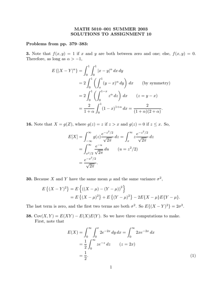
3. Note that f (x, y) = 1 if x and y are both between zero and one; else, f (x, y) = 0.
Therefore, as long as α > −1,
Z 1Z 1
α
E {|X − Y | } =
|x − y|α dx dy
0
0
Z 1 Z 1
α
=2
(y − x) dy dx
(by symmetry)
0
Z
1
x
1−x
Z
=2
α
z dz
0
2
=
1+α
Z
0
1
0
dx
(1 − x)1+α dx =
(z = y − x)
2
.
(1 + α)(2 + α)
16. Note that X = g(Z), where g(z) = z if z > x and g(z) = 0 if z ≤ x. So,
Z ∞ −z2 /2
2
e−z /2
e
g(z) √
z √
dz =
dz
E[X] =
2π
2π
−∞
x
Z ∞ −u
e
√ du
=
(u = z 2 /2)
2π
x2 /2
Z
∞
2
e−x /2
.
= √
2π
30. Because X and Y have the same mean µ and the same variance σ 2 ,
n
o
2
E (X − Y )2 = E ((X − µ) − (Y − µ))
= E (X − µ)2 + E (Y − µ)2 − 2E{X − µ}E{Y − µ}.
The last term is zero, and the first two terms are both σ 2 . So E{(X − Y )2 } = 2σ 2 .
38. Cov(X, Y ) = E(XY ) − E(X)E(Y ). So we have three computations to make.
First, note that
Z ∞Z x
Z ∞
−2x
E(X) =
2e
dy dx =
2xe−2x dx
0
0
Z 0
1 ∞ −z
=
ze dz
(z = 2x)
2 0
1
= .
2
1
(1)
Similarly,
Z
∞
Z
x
2y −2x
E(Y ) =
dy dx =
e
x
0
0
Z ∞
1
=
xe−2x dx = .
4
0
Finally,
Z
∞
Z
x
E(XY ) =
−2x
2ye
0
Z
=
0
∞
Z
∞
0
∞
dy dx =
xe−2x dx =
Z
x
y dy
dx
0
(2)
Z
0
2 −2x
e
x
−2x
Z
2e
0
x
y dy
dx
0
1
.
4
Therefore, this and equatinos (1) and (2), together yield: Cov(X, Y ) =
1
4
−
1
2
·
1
4
= 18 .
75. Because MY (t) = exp(2et − 2) and MX (t) = ( 14 + 34 et )10 (note the typo in some of
your texts), you can recognize the distribution of X as binomial with n = 10 and p = 34 ,
and that of Y as Poisson with λ = 2. Now to our regular programming · · ·
75. (a) X and Y are positive integers (albeit random variables), so that X + Y can only
be 2 if {X = 0, Y = 2}, {X = 1, Y = 1}, or {X = 2, Y = 0}. Therefore,
P {X + Y = 2} = P {X = 0} · P {Y = 2} + P {X = 1} · P {Y = 1}
+ P {X = 2} · P {Y = 2}
0 10
1 9
2
10
3
10
3
1
1
21
−2 2
=
+
·e
· e−2
0
1
4
4
2!
4
4
1!
2 8
10
3
1
20
· e−2
+
2
4
4
0!
467
= 10 2 = 0.000059.
4 e
76. We are asked to find MX,Y (s, t) = E{esX+tY } for all s and t. Let Z denote the
outcome of the second die and note that Y = X + Z. Therefore,
o
n
o
n
sX+t(X+Z)
(s+t)X tZ
=E e
e
MX,Y (s, t) = E e
= MX (s + t)MZ (t).
But X and Z have the same distribution, so
MX,Y (s, t) = MX (s + t)MX (t).
(3)
It remains to find the function MX . But this is easy: For any real number r,
6
rX er + e2r + · · · + e6r
1X r j
=
=
(e ) .
MX (r) = E e
6
6 j=1
2
(4)
This is a geometric sum, which
Pn
Pn I evaluate next.
Recall that for any u, j=0 uj = (un+1 − 1)/(u − 1). Therefore, j=1 uj = (un+1 −
1)/(u − 1) − 1 = (un+1 − u)/(u − 1) = u(un − 1)/(u − 1). Thanks to (4) (with u = er ),
1 er (enr − 1)
MX (r) =
.
6
er − 1
(5)
Use (3), and apply (5), once with r = s + t and once with r = t, to obtain:
"
#
et (ent − 1)
1 es+t en(s+t) − 1
MX,Y (s, t) =
.
36
es+t − 1
et − 1
77. (a) We want
MX,Y (s, t) = E esX+tY
Z ∞Z ∞
−y −(x−y)2 /2
e
sx+ty e
√
=
e
dx dy
2π
0
−∞
Z ∞Z ∞
−y −z 2 /2
e
s(z+y)+ty e
√
=
dz dy
(z = x − y)
e
2π
0
−∞
!
Z ∞
Z ∞
−z 2 /2
−[1−(s+t)]y
sz e
=
dz dy.
e
e √
2π
0
−∞
Now, the inside integral equals E(esZ ) where Z is N (0, 1). Therefore, this term is equal
to exp(s2 /2). Thus,
s2 /2
Z
∞
MX,Y (s, t) = e
e−[1−(s+t)]y dy
0

2

es /2

, if s + t < 1,
= 1 − (s + t)


+∞,
otherwise.
Theoretical Problem from p. 391:
13 (a). Let Ij = 1Pif a record occurs at j, and else Ij = 0. We are asked to show that
n
E[I1 + · · · + In ] = j=1 (1/j). I will show that E[Ij ] = 1/j; this is equivalent to showing
that E(Ij ) = 1/j which I will prove next.
Note that E(Ij ) is the probability that Xj > max(X1 , . . . , Xj−1 ); the seemingly innocent strict inequality is due to the fact that the X’s are continuous (why does this follow?),
and is very important in what is about to happen.
3
Note that X1 , . . . , Xj are exchangeable; i.e., the joint density of (X1 , · · · , Xj ) is the
same as that of any (and all) of the following:
• (X1 , · · · , Xj−2 , Xj , Xj−1 );
• (X1 , · · · , Xj−3 , Xj , Xj−2 , Xj−1 );
..
.
• (Xj , X1 , · · · , Xj−1 ).
In particular, P {Xj > max(X1 , . . . , Xj−1 )} is the probability that, in any of the above
items, the last random variable is greater than the maximum of the first j − 1 rv’s. There
are j equal probabilities here. Moreover, they represent disjoint events whose union is
everything (since one of the X’s must be maximum–the continuity of the X’s is coming in
here; sort the logic out). This means that jE(Ij ) = 1, which is equivalent to saying that
E(Ij ) = 1/j, as asserted.
4