Complex Adaptive Systems: Energy, Information and Intelligence: Papers from the 2011 AAAI Fall Symposium (FS-11-03)
Automatic Verification and Validation of a
CAS Simulation of an Intensive Care Unit
Christopher N. Eichelberger, Mirsad Hadzikadic
Ognjen Gajic, Guangxi Li
The University of North Carolina at Charlotte
9201 University City Boulevard
Charlotte, NC 20223
The Mayo Clinic
200 First Street SW
Rochester, MN 55905
Abstract
days of life
support
Complex adaptive systems (CAS) promise to be useful
in modeling and understanding real-world phenomena,
but remain difficult to validate and verify (V&V). The
authors present an adaptive, tool-chain-based approach
to continuous V&V that allows the subject matter experts (SMEs) and modelers to interact in a useful manner. A CAS simulation of the ICU at the Mayo Clinic is
used as a working example to illustrate the method and
its benefits.
$/day
life support
costs
financial
incentives
$/QALY
providers’
decisions
patient
health
QoL and QALY
patient
wishes
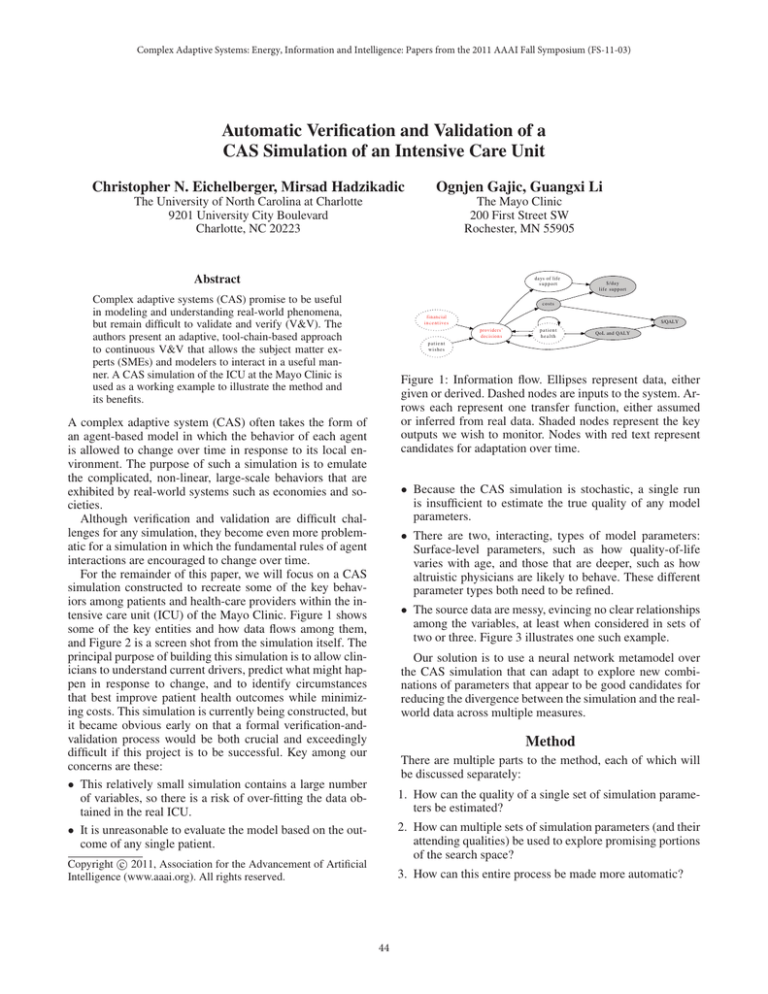
Figure 1: Information flow. Ellipses represent data, either
given or derived. Dashed nodes are inputs to the system. Arrows each represent one transfer function, either assumed
or inferred from real data. Shaded nodes represent the key
outputs we wish to monitor. Nodes with red text represent
candidates for adaptation over time.
A complex adaptive system (CAS) often takes the form of
an agent-based model in which the behavior of each agent
is allowed to change over time in response to its local environment. The purpose of such a simulation is to emulate
the complicated, non-linear, large-scale behaviors that are
exhibited by real-world systems such as economies and societies.
Although verification and validation are difficult challenges for any simulation, they become even more problematic for a simulation in which the fundamental rules of agent
interactions are encouraged to change over time.
For the remainder of this paper, we will focus on a CAS
simulation constructed to recreate some of the key behaviors among patients and health-care providers within the intensive care unit (ICU) of the Mayo Clinic. Figure 1 shows
some of the key entities and how data flows among them,
and Figure 2 is a screen shot from the simulation itself. The
principal purpose of building this simulation is to allow clinicians to understand current drivers, predict what might happen in response to change, and to identify circumstances
that best improve patient health outcomes while minimizing costs. This simulation is currently being constructed, but
it became obvious early on that a formal verification-andvalidation process would be both crucial and exceedingly
difficult if this project is to be successful. Key among our
concerns are these:
• This relatively small simulation contains a large number
of variables, so there is a risk of over-fitting the data obtained in the real ICU.
• It is unreasonable to evaluate the model based on the outcome of any single patient.
• Because the CAS simulation is stochastic, a single run
is insufficient to estimate the true quality of any model
parameters.
• There are two, interacting, types of model parameters:
Surface-level parameters, such as how quality-of-life
varies with age, and those that are deeper, such as how
altruistic physicians are likely to behave. These different
parameter types both need to be refined.
• The source data are messy, evincing no clear relationships
among the variables, at least when considered in sets of
two or three. Figure 3 illustrates one such example.
Our solution is to use a neural network metamodel over
the CAS simulation that can adapt to explore new combinations of parameters that appear to be good candidates for
reducing the divergence between the simulation and the realworld data across multiple measures.
Method
There are multiple parts to the method, each of which will
be discussed separately:
1. How can the quality of a single set of simulation parameters be estimated?
2. How can multiple sets of simulation parameters (and their
attending qualities) be used to explore promising portions
of the search space?
c 2011, Association for the Advancement of Artificial
Copyright Intelligence (www.aaai.org). All rights reserved.
3. How can this entire process be made more automatic?
44
o
o
250000
o
5
10
50000
model residual
+
0
5e+04
2e+04
5e+03
0
o
200000
o
o
o
o
o
o
oo
oo
o
o
o oooo o o
o+
o
o
o+
+ +
o
ooo
o
o
oo o o
+
oo
o+
o
o
++
oo
ooo
ooo+
+
o+
o
o
o oo+
o +
o
o
+
+
o
oo
ooo
o
o
o+
o
+
o
o
+
+
o
+
o
o+
+
+
o
o
++
o
o+
oo
oo+
o
o+
+
oo
+
oo
+
o
+
o
+
+
o
o
o
1e+04
(log) total cost of care
1e+05
o
o
150000
2e+05
o
o
100000
o
o invasive ventilation
+ no invasive ventilation
15
20
25
30
0
35
50000
100000 150000 200000 250000
actual cost
days of ventilation
Figure 3: Messy data. The left plot displays the wide variation in total patient cost against the number of days they
were on ventilation, separating those with invasive support
from those without. The left plot also includes a linear bestfit line, dashed, in red. The right plot displays the residuals
that result from applying this model.
Figure 2: Screen shot of the simulation running. The upperleft corner of the display indicates which medical provider
team is currently on duty. The lower-left corner is a legend.
The right side of the display shows the patients (as triangles)
who have been in the ICU within the most recent 7 days;
filled trianges are those on life support, while empty triangles are patients who are not on life support. Gray Xs represent patients who have died. As simulation time advances,
patients move from left to right, advancing through a week
in the ICU.
should approach zero asymptotically; exponential decay –
described by (2), and illustrated in Figure 4 – has precisely
this desirable quality.
Q = e−kΔ
Estimating quality of a single set of model
parameters
k=−
ln Qk
,
Δk
Q k , Δk > 0
(2)
(3)
The constant, k is merely a way to control the speed of the
decay. It is constrained by Δk and Qk , essentially the point
through which the quality curve must pass.
A CAS simulation is essentially a stochastic function that
accepts multiple input parameters, and produces multiple
outputs. Each variable, whether input or output, requires its
own metdata, including information about minimum values,
maximum values, and type. Outputs – at least those we will
use for training our simulation – will have observed values
from the real world. Even knowing, though, that mortality
will range from 0% to 100%, and is observed at 20% is not
enough to know how good a simulated value of 30% is.
This problem is more easily considered in two cases: 1) in
which we consider only a single dimension (output); and 2)
in which we consider multiple dimensions simultaneously.
Multiple dimensions Metamodels commonly are used for
only a single output (Reis Dos Santos and Porta Nova 1999),
(Doebling et al. 2002).
To combine the quality estimates of multiple dimensions,
it was important to us to emphasize the quality of all parts
of the model simultaneously. In an additive model, in which
the individual qualities are summed, excellent agreement in
one or more dimensions can mask gross disagreement in another. To reduce this tendency, we adopted a multiplicative
approach as described in (4).
One dimension It is reasonably easy to describe the divergence between the observation of a dimension’s value in
the real world and the simulated value for that dimension.
Though absolute or mean-squared error may be used (dos
Santos and dos Santos 2008), we chose an error fraction as
described in Equation (1). NB: This error measure may not
be useful for all metrics, but it works well for the outcome
measures within the ICU we are simulating.
|x −x |
rw
sim
if xrw > 0
xrw
(1)
Δ=
|xsim − xrw | otherwise
n Q = ∏ qmin + (1 − qmin ) · e−ki Δi wi
(4)
i
where qmin is a threshold value beneath which an individual
assessment is not allowed to fall (to prevent discontinuities
introduced by zeros), ki is defined as 80% of the reciprocal
range of the actual (observed) rate, and Δi is defined as the
absolute difference between the predicted rate and the actual
(observed) rate.
It can be difficult to visualize this relationship. As an
aid, consider that there are four principal dimensions against
which to benchmark simulation performance: 1) the mortality rate; 2) the cost per patient; 3) the number of quality life
years added (QALY); and 4) the cost per QALY. Allowing
where xsim the the simulated value for measure x, and xrw is
the value for measure x observed in the real-world data set.
Δ will be non-negative, ranging over [0, ∞). The fact that Δ
has no finite upper bound suggests that a quality function
45
158341
20 6
22279816
1 0000
0.6
0.8
1.0
0 981
0.0
0.2
0.4
Q
c=0 6931
0 000
0
1
2
3
4
0
00
0
0 0183
5
mortality (overal )
Δ
total cost ($)
QALY/patient
$/QALY
quality
Figure 5: Quality — the right-most column on the parallel
coordinates plot – as a function of the divergence of four
simulated rates from the actuals observed within the ICU at
the Mayo Clinic. Each variance is considered over the range
of 0% difference from the mean to 500% difference from the
mean: The actual, observed overall mortality rate, for example, is 19.6%, so the plot considers variance from 0% to approximately 98%. Colored lines represent combinations in
which the divergence for all four rates is less than or equal
to 100% of the observed value; combinations in which one
or more rates exhibits a variance of more than 100% are represented in shades of gray.
Figure 4: Exponential decay. In this plot, the X-axis represents the percentage divergence between a real dimension
and its simulated value. The Y-axis represents the quality
estimate assigned to that percent divergence. The decay is
constrained by the control point (100%, 0.5), highlighted by
the red cross-hairs; the decay constant that satisfies this constraint is 0.6931.
these four dimensions to assume variance from 0% to 500%
yields the overall quality estimates presented in Figure 5.
The figure shows that the majority of combinations of divergence across the dimensions map to relatively low estimates of overall quality. Only the combinations of uniformly
low divergence map to medium and high levels of quality for
the entire simulation. The purpose of this formulation is to
encourage the metamodel to raise the quality of all of the
constituent outputs in roughly equal measures.
As a practical example, we have also found that treating
these dimensions as large, high-level aggregates is not very
useful. When mortality is only considered (and controlled)
for the entire population, it encourages the simulation to
introduce odd behaviors within subgroups, such as having
the mortality rate decrease with age. If the sole purpose of
the simulation were to predict a single high-level aggregate
property, internal inconsistencies might not matter, but because we wish to allow clinicians to use the model to explore
ad hoc, these internal inconsistencies may become important. To minimize these variations, each of the four principal
dimensions is sub-divided into partitions based on sex and
age, and the total weights are apportioned among them. The
table 1 illustrates an example of the metrics for which the
original data from the Mayo Clinic contained enough cases
to be reliable:
The example data presented here result in an overall quality measure of approximately 60% according to the scoring
mechanism described previously.
selected parameter combinations, the metamodel is trained,
and asked to identify a single new point in the parameter
space that the data suggest might correspond with a lower
total error. This new point is the basis for a subsequent, relatively small, round of additional simulation rounds. The output of these additional simulations is added to the base data,
and the metamodel is retrained. This process is repeated until appropriate stop conditions are met.
We built our test harness so that it could use two separate
metamodels, each one method of training the CAS parameters: 1) using a traditional genetic algorithm (GA); 2) using
a neural network. The metamodels were applied similarity,
with accommodation made for their different requirements
(such as data encoding).
The experiments were controlled so that both methods
generated (and evaluated) the same number of candidates,
using the exact same evaluation routine. The evaluation routine ran each set of parameters through the simulation multiple times, so as to try to get a more representative estimation
of the output values than would result from any single run.
The purpose of the tests is to identify whether the blocksequential method of parameter-space exploration could be
effective, and to determine whether there are any important
differences in how the two metamodel paradigms respond.
Experiments
Results and discussion
An important consideration for metamodels is how to select the evaluation points that will be used as the training
cases (Wang 2005), (Kleijnen and Sargent 2000). For this
project, we are using sequential blocks of metamodel-guided
exploration. Starting with an initial sample of randomly-
Figure 6 demonstrates the results of a single run of the system. The GA behaves consistently, exhibiting the expected
pattern of punctuated equilibrium, while the neural network
appears to do a better job of identifying single, best solu-
46
metric
mortality, females, aged 65-74
mortality, females, aged 75-84
mortality, females, aged >=85
cost, females, aged 65-74
cost, females, aged 75-84
cost, females, aged >=85
QALY, females, aged 65-74
QALY, females, aged 75-84
QALY, females, aged >=85
$/QALY, females, aged 65-74
$/QALY, females, aged 75-84
$/QALY, females, aged >=85
mortality, males, aged 65-74
mortality, males, aged 75-84
mortality, males, aged >=85
cost, males, aged 65-74
cost, males, aged 75-84
cost, males, aged >=85
QALY, males, aged 65-74
QALY, males, aged 75-84
QALY, males, aged >=85
$/QALY males, aged 65-74
$/QALY, males, aged 75-84
$/QALY, males, aged >=85
weight
0.020
0.044
0.029
0.010
0.022
0.015
0.029
0.066
0.044
0.039
0.088
0.058
0.050
0.036
0.022
0.025
0.018
0.011
0.074
0.055
0.032
0.099
0.073
0.043
actual
0.1
0.34
0.42
27952
36532
22742
8.37
2.66
1.34
3338
13746
16985
0.17
0.31
0.43
30849
38000
28304
8.18
1.91
1.29
3771
19878
21884
simulated
0.28
0.32
0.30
43940
43429
43611
1.61
1.00
0.41
32784
522297
135203
0.30
0.29
0.30
42365
44645
42632
1.34
0.67
0.14
38418
81902
407738
Figure 6: Performance of the two metamodels contrasted.
There are four data series plotted: 1) the mean GA error (divergence) in blue; 2) the mean neural network error in yellow; 3) the best GA error in red; 4) the best neural network
error in green.
Table 1: An example of the metrics for which the original
data from the Mayo Clinic contained enough cases to be reliable.
Figure 7: Parallel coordinates plot mapping the exploration
of the parameter space by the two metamodels. Each line
represents a best-guess by the metamodel – trained on the
example seen so far – for what combination of parameters is
expected to yield the lowest error. The GA points are gray,
the neural network points are red, and the lowest-error point
is drawn in black.
tions. What is more subtle, and pehaps more important, is the
tendency of both mean-error lines to increase between significant discoveries. If the metamodels are exploring effectively, then they should be conducting experiments on novel
parameter combinations, most of which should perform relatively poorly, increasing the mean error over time, until a
break-through parameter combination is encountered.
The metamodeling process also brought to light another
minor finding, which is that the smoothness of the fitness
function appears to be directly related to the progression
of the error rates resulting from either metamodel. One of
the key advantages to the formulation of both the individual
and blended error rates may be the fact that they contain no
sharp discontinuities, no matter how large or unrealistic the
simulation errors become. This specific effect – unsurprising when one considers that both metamodels are rooted in
gradient descent – needs to be characterized quantitatively.
Figure 7 is a visualization of the parameter exploration
performed by the two metamodels. What the figure makes
very clear is the greater variety exhibited by the neural network metamodel. Whether the greater range of parameter
combinations is responsible for the neural network’s lower
error rate is not yet established. Because time is not represented in this visualization, the specific progression of the
exploration is lost.
The process described here is useful for much more than
simple parameter fitting, in as much as some of the fitted
parameter values brought to light shortcomings in the design
of the underlying simulation. Quality of life (QoL) is a good
example. The simulation contains an implicit model of how
QoL varies as a function of age, presuming an absolute scale.
The trained version of the two QoL parameters – QoL.a and
QoL.b – made it clear that the inferred model is wrong, and
motivated additional discussions between the modelers and
the clinicians. QoL is a relative, not absolute, scale, and the
simulation will be modified to accommodate this change.
The sub-divided outcome metrics appear to be helping
improve the deep quality of the simulation (as opposed to
the shallow, aggregate-only quality). The advantage this provides is that it reduces rounds of testing and refinement between the subject-matter experts (SMEs, clinicians in this
case) and the modelers. Automating these checks makes the
entire, iterative process faster and more efficient.
References
Barton, R. R. 2009. Simulation optimization using metamodels. In Winter Simulation Conference, WSC ’09, 230–
238. Winter Simulation Conference.
Caughlin, D. 1997. Automating the metamodeling process.
In Proceedings of the 29th conference on Winter simulation,
WSC ’97, 978–985. Washington, DC, USA: IEEE Computer Society.
Doebling, S. W.; Hemez, F. M.; Schultze, J. F.; and Cundy,
A. L. 2002. A metamodel-based approach to model vali-
47
dation for nonlinear finite element simulations. Proc. SPIE
4753:671–678.
dos Santos, M. I. R., and dos Santos, P. M. R. 2008. Sequential experimental designs for nonlinear regression metamodels in simulation. Simulation Modelling Practice and Theory.
Fishwick, P. 1989. Neural network models in simulation: A
comparison with traditional modeling approaches. In Simulation Conference Proceedings, 1989. Winter, 702 –710.
Fonseca, D. J.; Navaresse, D. O.; and Moynihan, G. P. 2003.
Simulation metamodeling through artificial neural networks.
Engineering Applications of Artificial Intelligence 16(3):177
– 183.
Jin, R.; Chen, W.; and Simpson, T. W. 2000. Comparative studies of metamodeling techniques under multiple modeling criteria.
In Proceedings of the 8th
AIAA/USAF/NASA/ISSMO Multidisciplinary Analysis &
Optimization Symposium.
Kilmer, R. A.; Smith, A. E.; and Shuman, L. J. 1995.
An emergency department simulation and a neural network
metamodel. Journal of the Society for Health Systems 63–
79.
Kleijnen, J. P., and Sargent, R. G. 2000. A methodology for
fitting and validating metamodels in simulation. European
Journal of Operational Research 120(1):14–29.
Mihram, G. A. 1970. An efficient procedure for locating
the optimal simular response. In Proceedings of the fourth
annual conference on Applications of simulation, 154–161.
Winter Simulation Conference.
Reis Dos Santos, M., and Porta Nova, A. 1999. The main issues in nonlinear simulation metamodel estimation. In Simulation Conference Proceedings, 1999 Winter, volume 1, 502
–509 vol.1.
Wang, L. 2005. A hybrid genetic algorithm-neural network
strategy for simulation optimization. Applied Mathematics
and Computation 170(2):1329 – 1343.
Yang, F. 2010. Neural network metamodeling for cycle
time-throughput profiles in manufacturing. European Journal of Operational Research 205(1):172–185.
48