Proceedings of the Twenty-Fifth International Florida Artificial Intelligence Research Society Conference
Social Influence Modeling for
Utility Functions in Model Predictive Control
Timothy Dockins and Manfred Huber
The University of Texas at Arlington
500 UTA Blvd Room 640 ERB
Arlington, TX 75019-0015
timothy.dockins@mavs.uta.edu, huber@cse.uta.edu
Abstract
Socially-aware Model Predictive Controller
Control Loop
Social influence has no small effect on the preferences
and behavior of agents in a social space. Contrary to
rationality, we sometimes compromise our own needs
for those of others. Thus, social influence has important implications in agent cognitive modeling for multiobjective decision-making problems. Namely, where
these activities occur within a social context, the intentional preferences or utility of an agent may be subsumed, to a greater or lesser degree, by the influences of
other agents. In this paper, a socially-aware model predictive controller is proposed using a social influence
network theory and applied to a HVAC control problem. It transforms individual agent utility to sociallyinfluenced utility reflecting interagent influences due to
their existing relationships.
MPC
Predictive Loop
Shared
Social
Space
Predictive
Models
Raw
Utility
Function
Social Influence Network
(Socially-Influenced Utility)
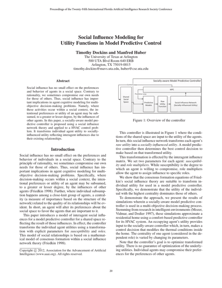
Figure 1: Overview of the controller
This controller is illustrated in Figure 1 where the conditions of the shared space are input to the utility of the agents.
In turn, this social influence network transforms each agent’s
raw utility into a socially-influenced utility. A model predictive controller then determines the best control decision to
make based on that transformed utility.
This transformation is effected by the interagent influence
matrix. We set two parameters for each agent: susceptibility and role multipliers. While susceptibility is the degree to
which an agent is willing to compromise, role multipliers
allow the agent to assign influence to specific roles.
We show that the consensus formation equations of Friedkin’s social influence theory are suitable to transform individual utility for used in a model predictive controller.
Specifically, we demonstrate that the utility of the individual with the highest centrality dominates those of others.
To demonstrate the approach, we present the results of
simulations wherein a socially-aware model predictive controller is used in a multi-objective decision-making process.
Stemming from research in intelligent environments (Mozer,
Vidmar, and Dodier 1997), these simulations approximate a
residential home using a comfort-based predictive controller
for its HVAC system. An occupying agent’s utility provides
input to the socially-aware controller which, in turn, makes a
control decision that modifies the thermal conditions inside
the home. The centrality of one agent (considered in the dependent role) is varied by changing its parameters.
Note that the controller’s goal is to optimize transformed
utility. There is no guarantee of optimization of the underlying utilities. Individual agents may compromise their preferences for the preferences of other agents.
Introduction
Social influence has no small effect on the preferences and
behavior of individuals in a social space. Contrary to the
principle of rationality, we sometimes compromise our own
needs for those of others. Thus, social influence has important implications in agent cognitive modeling for multiobjective decision-making problems. Specifically, where
decision-making occurs within a social context, the intentional preferences or utility of an agent may be subsumed,
to a greater or lesser degree, by the influences of other
agents (Friedkin 1998). Further, where individual subsumption happens among a close-knit group of agents, a centrality (a measure of importance based on the structure of the
network) related to the quality of its relationships will be evident. In short, an agent will alter its preferences about the
social space to favor the agents that are important to it.
This paper introduces a model of interagent social influences for a model predictive controller for a shared space reflecting the result of those influences. In effect, the controller
transforms the individual agent utilities using a transformation with explicit parameters for susceptibility and roles.
This model of social relationships is based on a mathematical model of consensus formation within a social influence
network theory (Friedkin 1998).
c 2012, Association for the Advancement of Artificial
Copyright Intelligence (www.aaai.org). All rights reserved.
20
Background
Notably, the prevalent standard measure of thermal comfort is the ASHRAE-scale based on a Predicted Mean Vote
(PMV) (ASHRAE 2004). The PMV indicates the expected
thermal comfort sensation of a large group of people on a
scale ranging from -3 to +3 reflecting sensations of cold and
hot, respectively. A neutral thermal comfort score on this
scale (PMV = 0) is from a combination of environmental and
individual factors for which no change is desired. The factors contributing to the comfort response of the individual
are given as four environmental variables (relative humidity, mean radiant temperature, ambient air temperature,air
velocity) and two personal variables (metabolic rate and
clothing levels). This is discussed briefly in (Liang and Du
2005) and a full treatment may be found in (ASHRAE 2004;
Fanger 1970).
Social influence network theory
Social influence network theory contains a formula for the
formation of consensus that ”describes a process in which
a group of actors weigh and integrate the conflicting influences of significant others - within the context of social
structural constraints” (Friedkin 1998). This is a form of
compromise where an agent’s opinion is influenced by the
opinions of other agents. We take the view here that opinions are analogous to utility and can be represented by scalar
numbers as follows:
Let N agents share a space. Let X = [xik ] be an N × K
matrix of the exogenous factors of that space that influence
the agents. Let B = [bkm ] be a K×M matrix of coefficients.
In essence, if X are the conditions of the shared space from
which an agent derives its utility, B is the set of weights
(t)
placed on those conditions. Y (t) = [yim ] is an N ×M matrix
of M -dimensional preferences for N agents at time t. The
initial (at time 1) and influenced preferences at time t can
then expressed as:
Y (1) = XB
Y
(t)
Model predictive control
The term model-based predictive control (MPC) refers to a
range of strategies designed to optimize a control policy by
maximizing some utility function. These strategies can be
summarized by three components. These are the prediction
model, the objective function and the process of obtaining
the control law (Camacho and Bordons 2004).
(Mozer, Vidmar, and Dodier 1997) describes a model
predictive controller which forms the objective function in
terms of occupant discomfort and an energy cost both measured in dollars:
(1)
= AW Y
(t−1)
+ (I − A)Y
(1)
(2)
Here, Equation (2) describes the subsequent transformation of those opinions over time where A = [aii ] is a diagonal weight matrix indicating the influence coefficient of each
agent, i, and W = [wij ] is the weight matrix N ×N describing the influences of the agents on each other. The weight
wij indicates the influence of agent j on agent i. Equations
(3) and (4) constrain the weight matrix, while Equation (5)
describes a compromise relationship.
0 ≤ wij ≤ 1
X
wij = 1
J¯u =
e(ut ) + m̄u (xt )
(6)
t=t0 +1
(3)
where e is the energy cost and m is the ”misery” of the occupants in dollars. These are described by their respective,
underlying models. The model predictive controller then
makes predictions about all the possible control policies over
a receding, finite window of time. Executing the first control
decision, the models are updated and the cycle repeated.
At each time step in a discrete control scenario, the optimal control policy is found by maximizing a utility function
informed by prediction models over a finite-horizon. The
first control action is then executed, the models updated, and
the optimal policy recalculated.
Driven by industry, the application of MPC controllers is
found to be used in a number of areas dominated by manufacturing process control (Qin and Badgwell 1997). However, given the simplicity of the approach, it is suitable for
other scenarios such as HVAC control. Indeed, the use of an
MPC controller for HVAC control is also shown in (Mozer,
Vidmar, and Dodier 1997; Freire, Oliveira, and Mendes
2008; Hamdi and Lachiver 1998; Lei, Hongli, and Cai
2006). Notably, Friere (Freire, Oliveira, and Mendes 2008)
investigates the use of PMV as a cost function in the HVAC
control scenario. Also, (Mozer, Vidmar, and Dodier 1997;
Freire, Oliveira, and Mendes 2008) investigate optimization
of both thermal comfort and energy cost generally using
MPC.
(4)
j
wii = 1 − aii
tX
0 +k
(5)
The first term of Equation (2) forms the norm of the
group. The revised opinion is the weighted sum of the norm
at that timestep and the agent’s initial opinion represented
by the second term. These relative weights are determined
by the coefficient of the social influence for each agent, aii .
Thus, each agent’s own opinion is accorded some weight
at this level, though its opinion is also accounted for in the
norm.
Thermal comfort and control
The primary goal of HVAC (Heating, Ventilating and Air
Conditioning) is to create an environment that is comfortable
for its occupants. Thermal comfort is studied in psychology
as an attempt to understand individual occupant responses
to the physical environment. When considering a thermal
comfort neutrality as the physiological state where heat generation and heat dissipation are equal, a thermal comfort response is then seen as the psychological response to deviation around that state. How this is measured is still an active
research topic, but a standard is readily available in the engineering field.
21
Methodology
is defined here for the group of agents as the matrix A such
that 0 < aii < 1 and aij = 0, i 6= j.
Problem formulation
Role multipliers Role multipliers are a convenient way to
handle different classes of relationships. We assume that a
relationship with one agent may be different than a relationship with another agent. It is also assumed that an agent’s
self-weight changes depending on some quality of the relationship. To simplify this, we assume that relationships fall
into groups or roles. Each role then scales the effect each
alter agent in that relationship role will have on the agent.
(Mozer, Vidmar, and Dodier 1997) formulated an HVAC
control problem as a balance between an optimal setpoint
and energy cost. In contrast, the problem is devised here as
a set of divergent objectives combined into a consensus decision reflecting the effect of social influence. These objectives are individually modeled as the utility of each agent
and combined using an influence network. This section describes modifications to Friedkin’s consensus formation as it
is included into a model predictive controller.
Role
peer
dependent
caregiver
Socially-aware Model Predictive Controller
The basic model predictive controller is modified by changing the model of agent utility. Specifically, raw utility is
transformed into socially-influenced utility according to
Equation (8). The agent entity can be generalized as any entity that 1) shares the social space, 2) is impacted by control
decisions on that space, 3) has some utility related to the
state of that space. While this obviously may include people, this definition allows us to include other agents such
as HVAC equipment. For example, an air conditioner is impacted by control decisions in that such decisions may cause
the device to consume energy. Energy usage could then be
considered as the utility function for that agent. In contrast to
(Mozer, Vidmar, and Dodier 1997), the aggregate objective
function can be simplified as a weighted sum of the utilities.
Multiplier
0.25
1.0
0.25
Table 1: Sample Multiplier Settings
Agents represent each role as a scalar multiplier. Table 1
provides an example set of role multipliers. Theoretically,
each agent could model roles individually. For the present,
we assume that all agents use the same role multipliers.
Raw utility In this paper, a distinction is made between
the raw utility of each agent and the socially-influenced utility. A raw utility function maps the conditions of the shared
space to a set of preferences for a given agent. Here we denote the raw utility of the agents as vector ~x such that each
agent’s utility occupies the corresponding row’s value.
Individual preferences are encoded into this characteristic. Any variances between individuals regarding utility
based on the conditions of the shared space but independent
of other agents occupying this space are therefore handled
by the agent’s raw utility function.
Social Space
The context for the control scenario is called the social
space. Latané and Liu (Latané and Liu 1996) define social space as ”an intersubjective matrix of psychological distances based on physical and social reality that provides a
framework constraining how people are influenced by each
other.” In the example scenario of an HVAC control problem, the social space is defined by shared use of a physical
location or environment (e.g. a residential home). It can also
be defined by a shared fiscal responsibility for the energy use
incurred by running the HVAC equipment.
Socially-influenced utility Socially-influenced utility, on
the other hand, represents the preferences of the individual
when taking other agents into consideration.
To relate these to the mechanism from social influence
network theory, the raw utilities of all the agents in a social
space are considered as the initial opinion, x in Equation
(1). We revise Wquations (1) and (2) to reflect the interrelated social influences for a single time-step. These equations are then combined into a single form by substituting
B~x for Y (1) , because we assume that social influence is entirely internal to the agent. Therefore, the focus is on the
relationships and each agent’s internal cognition about its
relationships.
Social agents
Social agents are those agents which jointly occupy a social
space along one or more defining dimensions. In this work,
agents have the following characteristics:
Occupancy An agent either occupies the social space at
time t or it does not. In the HVAC problem, an agent away
from the physical space at a given point in time will not be
affected by any control decisions affecting the space in that
time step. In Equation (8) below, occupancy is represented
by a diagonal matrix B (t) where:
1 agent i occupies the space at time t
(t)
bii =
(7)
0 otherwise
Y 0 = AW B~x + (I − A)B~x
(8)
The influence network is represented by the weight matrix, W , according to the constraints given in (3), (4) and
(5). As shown, this matrix can be used as a transformation
function transforming a vector of individual utilities to a vector of utilities representing the effect of the influence of the
relationships between the individual.
At each interval, the weight matrix W is updated. While
susceptibility and role multipliers remain constant, the number of occupants of each role changes over time. W is
Susceptibility Susceptibility is defined in two ways. First,
each agent may be more or less susceptible to the influences
of the group norm. This is a form of compromise between
one’s own utility and the utility of other group members. It
22
0.29
Cg
Cg
0.14
0.57
Agent
1
2
3
0.29
0.14
0.00
0.00
Dep
Figure 2: Influence Network
updated through the exponential function in Equation (9).
Though any function could be used here we make the assumption that the rate at which self-weight changes is exponential in relation to the number of related agents in a given
role and the quality of the relationship roles.
u∈H
mu nu
3
0.57
0.57
1.00
Figure 2 illustrates the distribution of influence between
the agents. The network centrality can be calculated as the
sum of the weights on the outgoing influences. The caregiver
agents (Cg) both have centrality of 0.43, while the dependent
agent (Dep) has a centrality of 2.14. In effect, changes in the
dependent agent’s utility will have a larger influence on the
aggregate utility.
1.00
PH
2
0.14
0.29
0.00
Table 2: Example Weight Matrix
0.57
wii = e−k
1
0.29
0.14
0.00
Experiments
Model Predictive Control
In short, the outdoor space model provides the exogenous
input for the system in terms of external weather conditions.
The thermal space model then simulates the movement of
heat through building walls resulting in an ambient indoor
temperature. Utility functions for the individual agents then
give a response to the temperature measured in terms of
comfort (on a [0,1] scale). These are combined into a group
utility as a weighted linear sum across all agents. The controller maximizes that utility over a finite horizon. The first
control action of the optimal policy is implemented. Finally,
the predictive models are updated and the next interval repeats the process.
(9)
where H is a set of relationship roles. The function parameters are k, m and n, where m is a multiplier for each relationship role h and n is an N -dimensional vector describing
the number of agents in relationship role h opposite agent i.
The parameter k scales the effects of other agents globally.
This represents the individual susceptibility of the agent to
social influence. At k = 1.0, the agent is fully influenced by
each individual term given in the sum. Agents that are not
influenced by others have k = 0.
Once the self-weight is calculated, influence can then be
distributed to the other agents. Equation (10) takes the remaining influence and distributes it according to their role.
mv
wij = (1 − wii ) P
(10)
h∈H mh nh
Predictive Models The social space is conceptualized
as a single-room having walls and ceiling with consistent
thermal resistance/capacitance. It is represented as ambient indoor temperature with a heat transfer equation. As
in (Mozer, Vidmar, and Dodier 1997), the transfer of heat
through the walls is modeled by a first-order approximation.
This is given by Equation (11).
−60δ
−60δ
ĥu (t) = ĥu (t − 1)e RC + (RQu(t) + g) 1 − e RC
where v is the relationship role of agent j vis-a-vis agent i.
Example
(11)
Consider a network with three agents; two agents (1 and 2)
are peers of each other and the other agent (3) is the dependent of the first two. This simulates two adults with a
dependent child in the HVAC problem.
Assuming k1 = 1.0, self-weight for agent 1 can be set as
follows:
This gives a prediction of the indoor temperature at time
t. Parameters, R and C are respectively the resistance and
capacitance factors. The equation is quantized by the interval size, δ. Finally, the current control decision (1 for heat,
0 for off, -1 for cool) is given by u while g is the outdoor
temperature.
Occupancy is represented in the present work using a
schedule-based model. For this report, each person agent
was given a daily period of not occupying the physical space
that randomly ranged between 4 and 12 hours.
Agent utility is represented differently based on agent
type. This work distinguishes the agents as either person
agents or thermal plant agents. Person agents are impacted
by the effects of the thermal environment and provide utility
in terms of thermal comfort. Thermal plant agents affect the
thermal environment and provide utility in terms of energy
usage. Both utilities are scaled to the [0,1] interval.
w11 = e−1.0×((1.0×1)+(0.25×1))
= 0.29
P
Given (1 − wii ) =
j6=i wij , the remaining 0.71 is distributed to the other agents according to (10). This maintains the constraints given in (3), (4), (5). Assume the same
weights for agent 2.
Let k3 = 0.0 give the susceptibility for agent 3. Trivially,
the self-weight for this agent will be 1.0 with none allocated
to agents 1 and 2. This results in the weight matrix, W , in
Table 2.
23
Agent
1
2
3
Thermal comfort utility is derived using fuzzy logic to
map indoor temperature to a PMV score. This is a rough
approximation of the method used in (Hamdi and Lachiver
1998) which provides a fast calculation of that score for online usage in HVAC controllers.
To demonstrate the suitability of this approach to the MPC
scenario, it suffices to show that the preferences of agents
with greater weighted centrality dominate the social space.
In this application, this means the more important an agent
is (i.e. greater centrality), the more comfortable it is. To
demonstrate, three simulations using different configurations of susceptibility were run. Each simulation consisted
of thirty trials. Between each trial, the thermal comfort and
occupancy profiles for each agent were varied randomly.
40 00
0.05
35 00
0.10
30 00
0.15
25 00
0.20
20 00
0.25
15 00
0.30
10 00
0.35
5.00
0.40
0.00
0.45
-5.00
0.50
1/1/2010
Agent 1
Agent 2
Agent 3 (DEP)
External Temp
Internal Temp
-10 00
2/1/2010 3/1/2010
4/1/2010
5/1/2010
6/1/2010
7/1/2010
8/1/2010
9/1/2010 10/1/2010
Figure 3: Simulation results for configuration 1
3
dependent
dependent
self
Configuration 2
For configuration 2, the agents in the caregiver roles had susceptibility parameter set to 0.5 (k = 0.5) while the dependent agent remained at k = 0.0. The recorded data is shown
in Table 5 and Figure 4(a).
Table 3: Agent Relationships
Each trial consists of 52,560 decision points (i.e. every
10 minutes for 12 months). At each decision point, external
temperature was used as input and the following output was
captured:
1.
2.
3.
4.
5.
0.00
Temperature (°C)
Discomfort Utility
Some parameters were commonly used across all configurations. Firstly, all simulations used three agents in a social
network whose relationships are described by Table 3. Also,
each agent used the role multipliers shown in Table 1. Finally, for all simulations, the dependent agent’s susceptibility parameter is set to zero for all simulations.
2
peer
self
caregiver
Std Dev (+)
0.01
0.02
0.02
Susceptibilities: 0.0,0.0,0.0
Common Configuration Parameters
1
self
peer
caregiver
Std Dev (-)
0.06
0.04
0.02
Table 4: Configuration 1 results
Data
Agent
1
2
3
Mean Utility
0.11
0.10
0.07
Agent
1
2
3
internal temperature
control decision (off, heat, cool)
agent’s occupancy status
agent’s raw utility
agent’s influenced utility
Mean Utility
0.04
0.07
0.04
Std Dev (-)
0.02
0.03
0.02
Std Dev (+)
0.02
0.01
0.01
Table 5: Configuration 2 results
Configuration 3
Exogenous Data
For configuration 3, the agents in the caregiver roles had susceptibility parameter set to 1.0 (k = 1.0) while the dependent agent remained at k = 0.0. The recorded data is shown
in Table 6 and Figure 4(b).
External temperature data was provided by NOAA data files
for Fayetteville, Arkansas (NOAA-NCDC 2011). Median
temperature was 17.4◦ C, minimum was −13.0◦ C and the
maximum was 43.0◦ C.
Discussion
Results
Importance in the social space is derived from the selfweight of the agent. We use the susceptibility parameter and
role multipliers to set that weight. The results shown above
indicate that as caregiver agent susceptibility increases, its
centrality increases and therefore its utility decreases. Further, the daily averages increase for the dependent agent as
the caregivers give more influence to it by increasing susceptibility.
The section provides the daily mean values for each decision
point index across all thirty trials.
Configuration 1
For configuration 1, the agents in the caregiver roles had susceptibility parameter set to 0.0 (k = 0.0). The recorded data
is shown in Table 4 and Figure 3.
24
40.00
-0.05
35.00
-0.05
35.00
-0.10
30.00
-0.10
30.00
-0.15
25.00
-0.15
25.00
-0.20
20.00
-0.20
20.00
-0.25
15.00
-0.30
10.00
Discomfort Utility
0.00
Agent 1
Agent 2
-0.25
15.00
-0.30
10.00
-0.35
5.00
-0.35
5.00
-0.40
0.00
-0.40
0.00
Agent 3 (DEP)
External Temp
Internal Temp
-0.45
5.00
-0.45
-0.50
1/1/2010
10.00
-0.50
1/1/2010
2/1/2010 3/1/2010
4/1/2010
5/1/2010
6/1/2010
7/1/2010
8/1/2010
9/1/2010 10/1/2010
(a) Configuration 2
Temperature (°C)
Susceptibilities: 1.0,1.0,0.0
40.00
Temperature (°C)
Discomfort Utility
Susceptibilities: 0.5,0.5,0.0
0.00
Agent 1
Agent 2
Agent 3 (DEP)
External Temp
Internal Temp
5.00
10.00
2/1/2010 3/1/2010
4/1/2010
5/1/2010
6/1/2010
7/1/2010
8/1/2010
9/1/2010 10/1/2010
(b) Configuration 3
Figure 4: Agent utility results for configurations 2 (a) and 3 (b)
Agent
1
2
3
Mean Utility
0.10
0.11
0.02
Std Dev (-)
0.04
0.05
0.00
Std Dev (+)
0.02
0.01
0.01
References
ASHRAE. 2004. ANSI/ASHRAE Standard 55R - Thermal
Environmental Conditions for Human Occupancy. Technical report, ASHRAE, Inc., Atlanta.
Camacho, E., and Bordons, C. 2004. Model predictive control. Springer Verlag, 2nd edition.
Fanger, P. 1970. Thermal comfort: analysis and applications
in environmental engineering. New York: McGraw-Hill.
Freire, R.; Oliveira, G.; and Mendes, N. 2008. Predictive
controllers for thermal comfort optimization and energy savings. Energy and Buildings 40(7):1353–1365.
Friedkin, N. 1998. A Structural Theory of Social Influence.
New York: Cambridge University Press.
Hamdi, M., and Lachiver, G. 1998. A fuzzy control system based on the human sensation of thermal comfort. In
Fuzzy Systems Proc., 1998. IEEE World Congress on Computational Intelligence., volume 1, 487–492. IEEE.
Latané, B., and Liu, J. 1996. The intersubjective geometry
of social space. Journal of Communication 46(4):26–34.
Lei, J.; Hongli, L.; and Cai, W. 2006. Model Predictive
Control Based on Fuzzy Linearization Technique For HVAC
Systems Temperature Control. 2006 1ST IEEE Conference
on Industrial Electronics and Applications 1–5.
Liang, J., and Du, R. 2005. Thermal comfort control based
on neural network for hvac application. Control Applications, 2005. CCA 2005. Proceedings of 2005 IEEE Conference on (Aug 819–824.
Mozer, M.; Vidmar, L.; and Dodier, R. H. 1997. The
Neurothermostat - Predictive Optimal Control of Residential Heating Systems. Advancements in Neural Info. Proc.
Systems 9:953–959.
NOAA-NCDC 2011. ASOS data (Fayetteville, AR; fiveminute resolution). www.ncdc.noaa.gov/
Qin, S., and Badgwell, T. 1997. An overview of industrial
model predictive control technology. Automatica.
Table 6: Configuration 3 results
This work has focused on the framework for a HVAC
scenario but it could be generalized to other control problems where a controller makes decisions on a shared, social
space. Other such controllers include recommender systems
for shared spaces such as media playlists.
Further, susceptibilities could be abstracted more to provide a robust and flexible system for parameterizing different susceptibilities to different exogenous inputs. In this
way, the utility of each agent could be more thoroughly described in the formalisms presented in Friedkin’s consensus
formation, rather than outside the system. That is to say that
an agent may also be more or less susceptible to the effects
of the different dimensions of the social space. For this work,
we assumed this susceptibility to be handled by the function
generating the utility. However, this could also be handled
by the matrix B by setting 0 < bij < 1 accordingly.
Finally, this work provides a platform for learning the parameters from some form of feedback from the agents. Exploration of this goal would require extending the cognitive
model of the agent in the simulator to provide appropriate
feedback to the socially-aware controller. A full, humanbased study would also serve the purpose.
Acknowledgments
This material is based upon work supported by the National
Science Foundation under Grant No. CNS-0649229.
25