Proceedings of the Fourteenth International Conference on Principles of Knowledge Representation and Reasoning
Strong Equivalence of Non-Monotonic Temporal Theories∗
Pedro Cabalar and Martı́n Diéguez
Dept. of Computer Science
University of Corunna, Spain
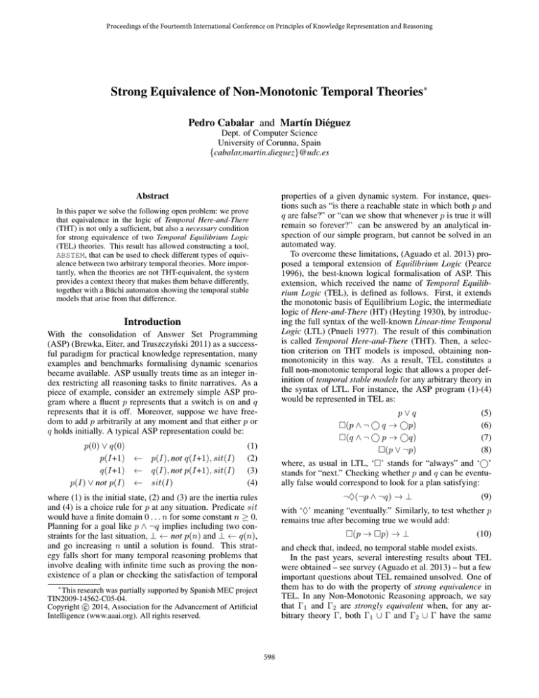
{cabalar,martin.dieguez}@udc.es
Abstract
properties of a given dynamic system. For instance, questions such as “is there a reachable state in which both p and
q are false?” or “can we show that whenever p is true it will
remain so forever?” can be answered by an analytical inspection of our simple program, but cannot be solved in an
automated way.
To overcome these limitations, (Aguado et al. 2013) proposed a temporal extension of Equilibrium Logic (Pearce
1996), the best-known logical formalisation of ASP. This
extension, which received the name of Temporal Equilibrium Logic (TEL), is defined as follows. First, it extends
the monotonic basis of Equilibrium Logic, the intermediate
logic of Here-and-There (HT) (Heyting 1930), by introducing the full syntax of the well-known Linear-time Temporal
Logic (LTL) (Pnueli 1977). The result of this combination
is called Temporal Here-and-There (THT). Then, a selection criterion on THT models is imposed, obtaining nonmonotonicity in this way. As a result, TEL constitutes a
full non-monotonic temporal logic that allows a proper definition of temporal stable models for any arbitrary theory in
the syntax of LTL. For instance, the ASP program (1)-(4)
would be represented in TEL as:
In this paper we solve the following open problem: we prove
that equivalence in the logic of Temporal Here-and-There
(THT) is not only a sufficient, but also a necessary condition
for strong equivalence of two Temporal Equilibrium Logic
(TEL) theories. This result has allowed constructing a tool,
ABSTEM, that can be used to check different types of equivalence between two arbitrary temporal theories. More importantly, when the theories are not THT-equivalent, the system
provides a context theory that makes them behave differently,
together with a Büchi automaton showing the temporal stable
models that arise from that difference.
Introduction
With the consolidation of Answer Set Programming
(ASP) (Brewka, Eiter, and Truszczyński 2011) as a successful paradigm for practical knowledge representation, many
examples and benchmarks formalising dynamic scenarios
became available. ASP usually treats time as an integer index restricting all reasoning tasks to finite narratives. As a
piece of example, consider an extremely simple ASP program where a fluent p represents that a switch is on and q
represents that it is off. Moreover, suppose we have freedom to add p arbitrarily at any moment and that either p or
q holds initially. A typical ASP representation could be:
p(0) ∨ q(0)
p(I+1) ← p(I), not q(I+1), sit(I)
q(I+1) ← q(I), not p(I+1), sit(I)
p(I) ∨ not p(I) ← sit(I)
p∨q
(p ∧ ¬ q → p)
(q ∧ ¬ p → q)
(p ∨ ¬p)
(1)
(2)
(3)
(4)
(5)
(6)
(7)
(8)
where, as usual in LTL, ‘’ stands for “always” and ‘’
stands for “next.” Checking whether p and q can be eventually false would correspond to look for a plan satisfying:
¬♦(¬p ∧ ¬q) → ⊥
where (1) is the initial state, (2) and (3) are the inertia rules
and (4) is a choice rule for p at any situation. Predicate sit
would have a finite domain 0 . . . n for some constant n ≥ 0.
Planning for a goal like p ∧ ¬q implies including two constraints for the last situation, ⊥ ← not p(n) and ⊥ ← q(n),
and go increasing n until a solution is found. This strategy falls short for many temporal reasoning problems that
involve dealing with infinite time such as proving the nonexistence of a plan or checking the satisfaction of temporal
(9)
with ‘♦’ meaning “eventually.” Similarly, to test whether p
remains true after becoming true we would add:
(p → p) → ⊥
(10)
and check that, indeed, no temporal stable model exists.
In the past years, several interesting results about TEL
were obtained – see survey (Aguado et al. 2013) – but a few
important questions about TEL remained unsolved. One of
them has to do with the property of strong equivalence in
TEL. In any Non-Monotonic Reasoning approach, we say
that Γ1 and Γ2 are strongly equivalent when, for any arbitrary theory Γ, both Γ1 ∪ Γ and Γ2 ∪ Γ have the same
∗
This research was partially supported by Spanish MEC project
TIN2009-14562-C05-04.
c 2014, Association for the Advancement of Artificial
Copyright Intelligence (www.aaai.org). All rights reserved.
598
def
selected models (stable models in ASP). (Lifschitz, Pearce,
and Valverde 2001) proved that checking equivalence in the
logic of HT is a necessary and sufficient condition for strong
equivalence in Equilibrium Logic, that is, Γ1 and Γ2 are
strongly equivalent iff Γ1 ≡HT Γ2 . A pair of strong equivalence checkers are, for instance, (Valverde 2004) and (Chen,
Lin, and Li 2005). This result for propositional HT was extended to arbitrary first-order theories in (Lifschitz, Pearce,
and Valverde 2007). It must be noticed that one direction
of this result, the sufficient condition, is actually trivial. As
HT is monotonic, Γ1 ≡HT Γ2 implies Γ1 ∪ Γ ≡HT Γ2 ∪ Γ
and so, their selected models will also coincide. The real
significant result is the opposite direction, namely, that HTequivalence is also a necessary condition for strong equivalence, as it shows that HT is strong enough as a monotonic basis for Equilibrium Logic. In the case of TEL,
(Aguado et al. 2008) implemented a prototype checker and
used it on some examples exploiting the trivial direction,
i.e., that THT-equivalence is obviously a sufficient condition
for strong equivalence in TEL. However, during the past six
years, the question whether THT-equivalence was also necessary or not remained unanswered.
In this paper we adapt a result from (Lifschitz, Pearce,
and Valverde 2007) to prove that indeed THT-equivalence
is a necessary condition for TEL strong equivalence and
use this proof, combined with previous theoretical results,
to construct a tool, ABSTEM1 , that allows the formal study
of arbitrary temporal theories in different ways. First, it
implements the technique in (Cabalar and Demri 2011) to
compute the temporal stable models of an arbitrary theory
Γ, displaying them as a Büchi automaton. Second, given
two theories Γ1 and Γ2 , it allows checking different types
of equivalence: LTL-equivalence, weak equivalence (coincidence in temporal stable models) and THT-equivalence
which, as said before, corresponds to strong equivalence.
The rest of the paper is organised as follows. In the next
section we recall the basic definitions of TEL. After that, we
overview the automata-based techniques from (Cabalar and
Demri 2011). The next section contains the main theorem.
This is followed by an explanation of the implementation
together with a practical example. Finally, we include some
conclusions.
usual propositional operators are defined as follows: ¬ϕ =
def
def
ϕ → ⊥, > = ¬⊥ and ϕ ↔ ψ = (ϕ → ψ) ∧ (ψ → ϕ).
Given a finite propositional signature At, an LTLinterpretation T is an infinite sequence of sets of atoms,
T0 , T1 , . . . with Ti ⊆ At for all i ≥ 0. Given two LTLinterpretations H, T we define H ≤ T as: Hi ⊆ Ti for
all i ≥ 0. A THT-interpretation M for At is a pair of
LTL-interpretations hH, Ti satisfying H ≤ T. A THTinterpretation is said to be total when H = T.
Definition 1 (Satisfaction) We define when an interpretation M = hH, Ti satisfies a formula ϕ at a state i ≥ 0,
written M, i |= ϕ, recursively as follows:
1. M, i |= p
2. ∧, ∨, ⊥
3. M, i |= ϕ → ψ
4. M, i |= ϕ
5. M, i |= ϕ U ψ
6. M, i |= ϕ R ψ
We say that hH, Ti is a model of a theory Γ, written
hH, Ti |= Γ, iff hH, Ti, 0 |= α for all formulas α ∈ Γ.
It is easy to see that restricting the study to total interpretations, THT-satisfaction collapses to LTL-satisfaction, i.e.:
Proposition 1 (from (Aguado et al. 2013)) hT, Ti, i |= ϕ
in THT iff T, i |= ϕ in LTL.
An interpretation M is a temporal equilibrium model of a
theory Γ if it is a total model of Γ, that is, M = hT, Ti |= Γ,
and there is no H < T such that hH, Ti |= Γ. An LTLinterpretation T is a temporal stable model (TS-model) of
a theory Γ iff hT, Ti is a temporal equilibrium model of Γ.
By Proposition 1 it is easy to see that any TS-model of a
temporal theory Γ is also an LTL-model of Γ.
As happens in LTL, the set of TS-models of a theory Γ can
be captured by a Büchi automaton (Büchi 1962), a kind of
ω-automaton (that is, a finite automaton that accepts words
of infinite length). In this case, the alphabet of the automaton would be the set of states (classical propositional interpretations) and the acceptance condition is that a word (a
sequence of states) is accepted iff it corresponds to a run of
the automaton that visits some acceptance state an infinite
number of times. As an example, Figure 1 shows the TSmodels for the theory (5)-(8) which coincide with sequences
of states of the forms {q}∗ {p}ω or {q}ω .
Temporal Equilibrium Logic
We begin defining the (monotonic) logic of THT as follows.
The syntax is defined as in propositional LTL. A temporal
formula ϕ can be expressed following the grammar shown
below:
ϕ ::= ⊥ | p | α ∧ β | α ∨ β | α → β | α | α U β | α R β
Computing Temporal Stable Models of
Arbitrary Theories
where p is an atom of some finite signature At, and α and β
are temporal formulas in their turn.
The formula α U β stands for “α until β” whereas α R β
is read as “α release β” and is the dual of “until.” Derived operators such as (“always”) and ♦ (“at some future
def
def
time”) are defined as ϕ = ⊥ R ϕ and ♦ϕ = > U ϕ. Other
1
iff p ∈ Hi , with p an atom.
as usual
iff for all x ∈ {H, T},
hx, Ti, i 6|= ϕ or hx, Ti, i |= ψ.
iff M, i+1 |= ϕ
iff ∃k ≥ i such that M, k |= ψ and
∀j ∈ {i, . . . , k-1}, M, j |= ϕ.
iff ∀k ≥ i such that M, k 6|= ψ then
∃j ∈ {i, . . . , k-1}, M, j |= ϕ. Based on the techniques introduced in (Cabalar and Demri
2011), the tool ABSTEM constitutes the first implementation
capable of computing TS-models for arbitrary temporal formulas, without syntactic restrictions. The method obtains
the TS-models of a formula ϕ by performing several operations on a pair of automata derived from ϕ. The first
automaton, denoted as Aϕ , accepts the total THT-models
http://kr.irlab.org/?q=abstem
599
{q}
Proposition 2 Let hH, Ti be a THT interpretation for signature At. If hH, Ti |= γ0 then H = T.
S1
Corollary 1 For any formula α for signature At, the LTLmodels of α ∧ γ0 coincide with its TS-models.
{p}
{q}
start
S0
{p}
Lemma 1 Let α and β be two LTL-equivalent formulas and
let γ = (β → γ0 ). Then, the following conditions are equivalent:
{p}
S2
Figure 1: Temporal stable models of theory (5)-(8).
(i) There exists some H < T such that hH, Ti 6|= α → β;
(ii) T is TS-model of β ∧ γ but not TS-model of α ∧ γ.
Theorem 2 (Main theorem: necessary condition) If two
temporal formulas α and β are strongly equivalent in TEL
then they are THT-equivalent.
hT, Ti of ϕ. By Proposition 1 this simply amounts to compute the LTL models T of ϕ using an automata construction method for LTL. The second automaton, denoted as
Aϕ00 , accepts the non-total THT-models hH, Ti of ϕ. The
final set of TS-models is obtained from the composition
Aϕ ∩ h(Aϕ00 ) where h(Aϕ00 ) filters out the H component of
non-total models, h(Aϕ00 ) is the complementary of h(Aϕ00 )
and finally ∩ denotes the automata product.
The computation of Aϕ00 is done exploiting a translation
of THT into LTL first presented in (Aguado et al. 2008)
and directly extrapolating the translation of HT into classical logic in (Pearce, Tompits, and Woltran 2001). It uses
an extended signature {p0 | p ∈ At} so that p0 represents the
truth of p in H while p is used for T. The translation of ϕ,
written ϕ∗ , is recursively defined as follows:
Proof We will prove that if α and β are not THT-equivalent
then there is some context formula γ for which α∧γ and β ∧
γ have different TS-models. Assume first that α and β have
different total models, i.e., different LTL-models. Then, the
LTL-models of α ∧ γ0 and β ∧ γ0 also differ (since γ0 is an
LTL tautology). But by Corollary 1, LTL-models of these
theories are exactly their TS-models, and so, they also differ.
Suppose now that α and β are LTL-equivalent but not
THT-equivalent. Then, there is some THT-countermodel
hH, Ti of either (α → β) or (β → α), and given LTLequivalence of α and β, the countermodel is non-total, H <
T. Without loss of generality, assume hH, Ti 6|= α → β.
By Lemma 1, taking the formula γ = (β → γ0 ), we get that
T is TS-model of β ∧ γ but not TS-model of α ∧ γ.
def
• (p)∗ = p0 , for any atom p ∈ At
Algorithm 1 StrongEquivalenceTest(α, β)
Require: Two propositional temporal formulas α, β.
Ensure: If α and β are THT-equivalent, it returns true.
Otherwise, it returns a triple hγ, A1 , A2 i.
def
• (α → β)∗ = (α → β) ∧ (α∗ → β ∗ )
being homomorphic for the rest of logical connectives. To
impose the restriction H < T we further include the axiom:
^
_
0
0
(p → p) ∧
♦(¬p ∧ p)
(Ax1)
p∈At
A1 := ltl to Büchi(α ∧ ¬β)
A2 := ltl to Büchi(β ∧ ¬α)
if A1 6= ∅ or A2 6= ∅ then
return hγ0 , A1 , A2 i
end if
A=ltl to Büchi(¬(α → β)∗ ∧ (Ax1))
if A 6= ∅ then
A2 := h(A)
return h(β → γ0 ), ∅, A2 i
end if
A=ltl to Büchi(¬(β → α)∗ ∧ (Ax1))
if A 6= ∅ then
A1 := h(A)
return h(α → γ0 ), A1 , ∅i
end if
return true
p∈At
def
Automaton Aϕ00 is built from formula ϕ00 = ϕ∗ ∧ (Ax1).
The operation h(Aϕ00 ) returns a new automaton that results
from removing the atoms p0 from transitions in Aϕ00 . This
captures the T-components of non-total models; in this way,
its complementary automaton h(Aϕ00 ) accepts the T sequences that do not form a non-total model, but perhaps they
are not models either. Thus, the final product Aϕ ∩ h(A00ϕ )
captures those T such that hT, Ti is a total model of ϕ and
no non-total model hH, Ti can be formed.
Temporal Strong Equivalence
For simplicity, we assume finite theories and we indistinctly
represent them as the conjunction of their formulas.
Theorem 1 (Sufficient condition (Aguado et al. 2008))
If two temporal formulas α and β are THT-equivalent then
they are strongly equivalent in TEL.
To prove the other direction, namely, that THTequivalence is also a necessary condition for strong equivalence, we begin defining γ0 as the conjunction of all formulas (p ∨ ¬p) for all atoms p ∈ At.
Implementation and a practical example
The procedure for checking strong equivalence in ABSTEM
is shown in Algorithm 1. It takes two arbitrary propositional
temporal formulas α and β and returns either true, if they
are strongly equivalent, or a triple with a formula γ and two
600
automata A1 , A2 otherwise2 . The meaning of this information is that A1 captures TS-models of α ∧ γ that are not TSmodels of β ∧ γ and, analogously, A2 captures TS-models
of β ∧ γ that are not TS-models of α ∧ γ. The procedure
uses an auxiliary routine ltl to Büchi(ϕ) to obtain a Büchi
automaton from an LTL-formula ϕ.
As an example of use, let β1 be our “switch” domain
(5)-(8) plus the rule (¬p → q) trying to capture the idea
that, when no information on p is available, q becomes true.
This new rule is actually a new default for q that interacts
with inertia rules (6),(7) destroying somehow their effect.
Using ABSTEM to check the TS-models of β1 we obtain
the automaton in Figure 2(a) which corresponds to arbitrary sequences formed with states {p} and {q}. This set
of TS-models actually coincides with what one would expect from a formula of the form (p ∨ q) since, as happens
in ASP, truth minimality converts the disjunction into an exclusive or. So, we may conjecture that β1 is equivalent to
α1 = (p ∨ q). Using ABSTEM we can check that, in fact,
α1 and β1 have the same TS-models and, furthermore, they
are also LTL-equivalent. However, α1 and β1 are not THTequivalent and so, they are not strongly equivalent. The answer displayed this time by ABSTEM is negative and shows
the context formula γ1 = β1 → γ0 plus a file containing the
automaton in Figure 2(b). This automaton captures all the
TS-models of β1 ∧ γ1 that are not TS-models of α1 ∧ γ1 .
counterexamples in the form of a Büchi automaton. Regarding efficiency and scalability, this prototype works satisfactorily for small theories like the ones presented in the paper.
It must be noted, however, that checking THT-equivalence
is a PS PACE-complete problem.
References
Aguado, F.; Cabalar, P.; Pérez, G.; and Vidal, C. 2008.
Strongly equivalent temporal logic programs. In JELIA’08,
volume 5293 of Lecture Notes in Computer Science, 8–20.
Aguado, F.; Cabalar, P.; Diéguez, M.; Pérez, G.; and Vidal,
C. 2013. Temporal equilibrium logic: a survey. Journal of
Applied Non-Classical Logics 23(1-2):2–24.
Brewka, G.; Eiter, T.; and Truszczyński, M. 2011. Answer
set programming at a glance. Commun. ACM 54(12):92–
103.
Büchi, R. 1962. On a decision method in restricted secondorder arithmetic. In Intl. Congress on Logic, Method and
Philosophical Science’60, 1–11.
Cabalar, P., and Demri, S. 2011. Automata-based computation of temporal equilibrium models. In Vidal, G., ed.,
LOPSTR’11, Lecture Notes in Computer Science. Odense,
Denmark: Springer.
Chen, Y.; Lin, F.; and Li, L. 2005. SELP - a system for
studying strong equivalence between logic programs. In LPNMR’05, volume 3662 of Lecture Notes in Computer Science, 442–446.
Heyting, A.
1930.
Die formalen Regeln der intuitionistischen Logik. Sitzungsberichte der Preussischen
Akademie der Wissenschaften, Physikalisch-mathematische
Klasse 42–56.
Lifschitz, V.; Pearce, D.; and Valverde, A. 2001. Strongly
equivalent logic programs. Computational Logic 2(4):526–
541.
Lifschitz, V.; Pearce, D.; and Valverde, A. 2007. A characterization of strong equivalence for logic programs with
variables. In LPNMR’07, volume 4483 of Lecture Notes in
Computer Science. Springer.
Pearce, D.; Tompits, H.; and Woltran, S. 2001. Encodings for equilibrium logic and logic programs with nested
expressions. In EPIA 2001, volume 2258 of Lecture Notes
in Computer Science, 306–320. Springer.
Pearce, D. 1996. A new logical characterisation of stable
models and answer sets. In NMELP’96, volume 1216 of
Lecture Notes in Artificial Intelligence. Springer. 57–70.
Pnueli, A. 1977. The temporal logic of programs. In
FOCS’77, 46–57. IEEE.
Valverde, A. 2004. tabeql: A tableau based suite for equilibrium logic. In JELIA’04, volume 3229 of Lecture Notes
in Artificial Intelligence, 734–737.
{p}, {q}, {p, q}
S1
{q}, {p}
{q},{p}
{p, q}
{p, q}
start
S0
(a) TS-models of
α1 and β1 .
start
S0
{q},{p}
S2
(b) TS-models of β1 ∧ γ1 not of α1 ∧ γ1 .
Figure 2: Temporal stable models related to α1 and β1 .
Conclusions
In this paper we have adapted (Lifschitz, Pearce, and
Valverde 2007) to the temporal case, to prove that equivalence in the logic of Temporal Here-and-There (THT), is not
only a sufficient but also a necessary condition for strong
equivalence in Temporal Equilibrium Logic (TEL). Using
this proof, we have implemented a system, ABSTEM, for
analysing TEL arbitrary theories in different ways. First,
ABSTEM constitutes the first tool for computing temporal
equilibrium models of any arbitrary temporal theory. Second, it also allows checking three types of equivalence between two arbitrary theories: LTL, weak and strong equivalence. When equivalence is not satisfied, ABSTEM shows
2
For further details, see the extended version of this document
at http://kr.irlab.org/sites/default/files/papers/kr2014-ex.pdf.
601