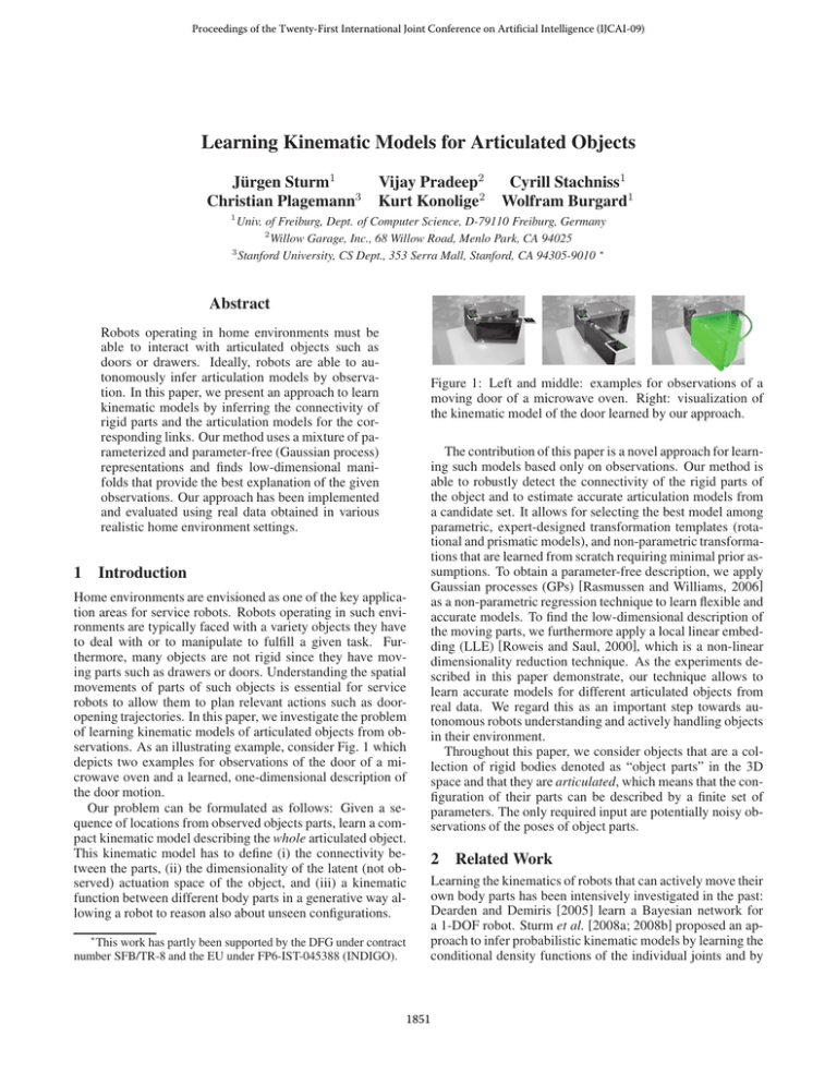
Proceedings of the Twenty-First International Joint Conference on Artificial Intelligence (IJCAI-09)
Learning Kinematic Models for Articulated Objects
Jürgen Sturm1
Christian Plagemann3
Vijay Pradeep2
Kurt Konolige2
Cyrill Stachniss1
Wolfram Burgard1
1
Univ. of Freiburg, Dept. of Computer Science, D-79110 Freiburg, Germany
2
Willow Garage, Inc., 68 Willow Road, Menlo Park, CA 94025
3
Stanford University, CS Dept., 353 Serra Mall, Stanford, CA 94305-9010 ∗
Abstract
Robots operating in home environments must be
able to interact with articulated objects such as
doors or drawers. Ideally, robots are able to autonomously infer articulation models by observation. In this paper, we present an approach to learn
kinematic models by inferring the connectivity of
rigid parts and the articulation models for the corresponding links. Our method uses a mixture of parameterized and parameter-free (Gaussian process)
representations and finds low-dimensional manifolds that provide the best explanation of the given
observations. Our approach has been implemented
and evaluated using real data obtained in various
realistic home environment settings.
Figure 1: Left and middle: examples for observations of a
moving door of a microwave oven. Right: visualization of
the kinematic model of the door learned by our approach.
1 Introduction
Home environments are envisioned as one of the key application areas for service robots. Robots operating in such environments are typically faced with a variety objects they have
to deal with or to manipulate to fulfill a given task. Furthermore, many objects are not rigid since they have moving parts such as drawers or doors. Understanding the spatial
movements of parts of such objects is essential for service
robots to allow them to plan relevant actions such as dooropening trajectories. In this paper, we investigate the problem
of learning kinematic models of articulated objects from observations. As an illustrating example, consider Fig. 1 which
depicts two examples for observations of the door of a microwave oven and a learned, one-dimensional description of
the door motion.
Our problem can be formulated as follows: Given a sequence of locations from observed objects parts, learn a compact kinematic model describing the whole articulated object.
This kinematic model has to define (i) the connectivity between the parts, (ii) the dimensionality of the latent (not observed) actuation space of the object, and (iii) a kinematic
function between different body parts in a generative way allowing a robot to reason also about unseen configurations.
∗
This work has partly been supported by the DFG under contract
number SFB/TR-8 and the EU under FP6-IST-045388 (INDIGO).
The contribution of this paper is a novel approach for learning such models based only on observations. Our method is
able to robustly detect the connectivity of the rigid parts of
the object and to estimate accurate articulation models from
a candidate set. It allows for selecting the best model among
parametric, expert-designed transformation templates (rotational and prismatic models), and non-parametric transformations that are learned from scratch requiring minimal prior assumptions. To obtain a parameter-free description, we apply
Gaussian processes (GPs) [Rasmussen and Williams, 2006]
as a non-parametric regression technique to learn flexible and
accurate models. To find the low-dimensional description of
the moving parts, we furthermore apply a local linear embedding (LLE) [Roweis and Saul, 2000], which is a non-linear
dimensionality reduction technique. As the experiments described in this paper demonstrate, our technique allows to
learn accurate models for different articulated objects from
real data. We regard this as an important step towards autonomous robots understanding and actively handling objects
in their environment.
Throughout this paper, we consider objects that are a collection of rigid bodies denoted as “object parts” in the 3D
space and that they are articulated, which means that the configuration of their parts can be described by a finite set of
parameters. The only required input are potentially noisy observations of the poses of object parts.
2 Related Work
Learning the kinematics of robots that can actively move their
own body parts has been intensively investigated in the past:
Dearden and Demiris [2005] learn a Bayesian network for
a 1-DOF robot. Sturm et al. [2008a; 2008b] proposed an approach to infer probabilistic kinematic models by learning the
conditional density functions of the individual joints and by
1851
subsequently selecting the most likely topology. Their approach requires knowledge about the actions carried out by
the robot or by the observed object—information which is
not available when learning the models of arbitrary, articulated objects from observations only. Similarly, Taycher
et al. [2002] address the task of estimating the underlying
topology of an observed articulated body. Their focus lies
on recovering the topology of the object rather than on learning a generative model with explicit action variables. Also,
compared to their work, our approach can handle higherdimensional transformations between object parts. Kirk et
al. [2004] extract human skeletal topologies using 3D markers from a motion capture system. However, they assume that
all joints are rotational.
Yan and Pollefeys [2006] present an approach for learning
the structure of an articulated object from feature trajectories
under affine projections. They first segment the feature trajectories by local sampling and spectral clustering and then
build the kinematic chain as a minimum spanning tree of a
graph constructed from the segmented motion subspaces.
Other researchers have addressed the problem of identifying different object parts from image data. Ross et al. [2008]
use multi-body structure from motion to extract links from
an image sequence and then fit an articulated model to these
links using maximum likelihood learning. There also exist approaches for identifying humans that assume a known
topology of the body parts. Ramanan [2006] perform pose estimation of articulated objects from images using an iterative
parsing approach. They seek to improve the feature selection
to better fit the model to the image.
There exist several approaches where tracking articulated
objects is the key motivation and often an a-priori model is assumed. Comport et al. [2004], for example, describe a framework for visual tracking of parametric non-rigid multi-body
objects based on an a-priori model of the object including a
general mechanical link description. Chu et al. [2003] present
an approach for model-free and marker-less model and motion capture from visual input. Based on volume sequences
obtained from image data from calibrated cameras, they derive a kinematic model and the joint angle motion of humans
with tree-structured kinematics.
Similar to our approach for identifying low-dimensional
articulation actions, Tsoli and Jenkins [2009] presented an
Isomap-based technique that finds a low-dimensional representation of complex grasp actions. This allows human operators to easily carry out remote grasping tasks.
Katz et al. [2008] learn planar kinematic models for articulated objects such as 1-DOF scissors or a 3-DOF snake-like
toy. They extract features from a series of camera images, that
they group together to coherently moving clusters as nodes in
a graph. Two nodes are connected in the graph when they are
rigid. Subsequently, rotational and prismatic joints are identified by searching for rotation centers or shifting movements.
In contrast to their work, we use 3D information and are not
restricted to prismatic and rotation joints. We additionally can
model arbitrary movements including those of garage doors
which are 1-DOF actions that cannot be described by a prismatic or rotational joint. The approach of Katz et al. [2008]
is furthermore focused on manipulation actions whereas our
approach is passive and only based on observations.
3 Learning Models of Actuated Objects
In this work, we consider articulated objects consisting of
n rigid object parts, which are linked mechanically as an
open kinematic chain. We assume that a robot, external to the
object, observes the individual parts and that it has no prior
knowledge about their connectivity.
To describe the kinematics of such an articulated object, we
need to reason about (i) the connections of the object parts
(the topology) and (ii) the kinematic nature of the connections. Our approach seeks to find the topology and the local models that best explain the observations. We begin with
a discussion of how to model the relationship of two object
parts. The extension towards an entire graph of parts and relations is then given in Section 3.3.
3.1
Modeling the Interaction between Two Parts
The state of an object part i can be described by a vector
xti ∈ R6 representing the position and orientation of the part
i ∈ 1, . . . , n at time t = 1, . . . , T . We assume that only their
relative transformation Δij = xi xj is relevant for estimating the model, where ⊕ and are the motion composition
operator and its inverse.
If the two object parts are not rigidly connected, we assume that the articulation can be described by a latent (not observed) action variable. Examples for a latent action variable
are the rotation angle of a door or the translation of a drawer.
The goal is now to describe the relative transformation between the object parts using such a latent variable aij ∈ Rd ,
where d represents the intrinsic DOF of the connection between i and j.
Since we have no prior information about the nature of the
connection, we do not aim to fit a single model but instead
aim to fit a set of candidate template models representing different kinds of joints. This candidate set consists of parameterized models that occur in various objects including a rotational joint (Mrotational ), a prismatic joint (Mprismatic ), and a
rigid transformation (Mrigid ). Additionally, there may be articulations that do not correspond to these standard motions,
for which we consider parameter-free models (MLLE/GP ).
These are computed by using a combination of the local linear
embedding (LLE) dimensionality reduction technique and a
Gaussian process. A more detailed description of these models is given in Section 3.4
1:T
We use a sequence of T noisy observations zij
=
1
T
zij , . . . , zij of Δij for fitting the candidate models and for
evaluating which model appears to be the best one. This is
done by performing 2-fold cross-validation. In the remainder of this paper, we refer to Dij as the training data selected
1:T
test
from the observations, where Dij ⊂ zij
, and to Dij
as the
(disjoint) set of test data.
3.2
Evaluating a Model
Let Mij be an articulation model p(Δij | a) describing the
connection between the part i and j and learned from the
training data Dij . To actually evaluate how well an observation zij can be explained by a model, we have to determine
1852
p(zij | Mij ) which corresponds to
p(zij | Mij ) = p(zij | a, Mij ) p(a | Mij ) d a.
(1)
a
The variable a is the latent action variable of the model that,
for example, describes the opening angle of a door.
We assume that during the observations, there is no latent
action state a that is more likely than another one, i.e., that
p(a | Mij ) is a uniform distribution. Note that this is an
approximation since in our door example, one might argue
that doors are more likely to be closed or completely opened
compared to other states. This assumption simplifies Eq. 1 to
(2)
p(zij | Mij ) = p(zij | a, Mij ) d a.
a
To evaluate p(zij | a, Mij ), that is, a measure for how well
model Mij parameterized by the action variable a explains
the observation zij of the part transformation Δij , we first
compute the expected transform
Δ̂ij = EMij [Δij | a] = fMij (a)
To actually compute p(zij | Mij ) using Eq. 2, we need to
compute the integral over the latent action variable a. In this
paper, we solve this by performing Monte-Carlo integration
by sampling multiple instances of the latent variable.
Since this procedure can be rather time-consuming, we also
tested an alternative strategy to approximate the integral. If
we assume that p(zij | a, Mij ) is unimodal, we can think of
evaluating it only at the most likely latent action variable and
approximate Eq. 2 by
max p(zij | a, Mij ).
a
(5)
Depending on the realization of the model Mij , we can carry
out the maximization step to compute p(zij | Mij ) efficiently.
Finally, we can compute the data likelihood for the test data
set
test
| Mij ) =
p(zij | Mij ).
(6)
p(Dij
test
zij ∈Dij
3.3
Mij ∈M
while at the same time minimizing the overall complexity of
the combined model. The latter is calculated in a fashion similar as with the Bayesian information criterion. In our case,
we measure the model complexity by the dimensionality of
the latent action space.
To find this topology (that is, the spanning tree of the local
models), we fit for all tuples of rigid parts all models from
the candidate template model set and add for each model a
link to the graph. We then assign to each edge in the graph
the cost of model Mtype
ij that is equal to the negative expected
data log-likelihood plus a complexity penalty of the model:
(3)
using a model-specific transformation function fMij (a). In
Section 3.4, we will specify this transformation function for
all model templates. Note that we reason about the relative
configuration between object parts here and compare the result to the observed transformation under a Gaussian error
assumption with variance σ 2 :
(4)
p(zij | a, Mij ) ∝ exp −||Δ̂ij − zij ||2 /σ 2
p(zij | Mij ) =
reasoning with all possible topologies, however, results in an
intractable complexity. We therefore seek to find the spanning tree M that results in a combined model for all object
parts that both maximizes the expected data likelihood of a
new observation, i.e.,
test
p(Dij
| Mij ),
(7)
p(Dtest | M) =
Finding the Connectivity
So far, we ignored the question of connectivity and described
how to evaluate a model Mij representing a connection between the parts i and j. If we consider the individual object
parts as nodes in a graph and the connections as edges between nodes, then the set of possible acyclic object structures
that connect all parts is given by all spanning trees of this
graph. The endeavor of explicitly computing, evaluating, and
costMtype = −
ij
1
type
type
log p(Dtest | Mij ) + C(Mij )
Dtest (8)
Then, the task of finding the topology of local models which
minimize this cost function is equivalent to finding the minimal spanning tree in this graph which can be done rather
efficiently.
Please note that the resulting kinematic tree can be transformed into a Bayes net (BN) by replacing the edges by connected nodes representing local models M and latent action
variables a and by adding nodes for (absolute) object part
observations and relative observations z. The resulting BN
naturally encodes all independence assumptions made in our
work. Such a BN, however, is complex and hard to visualize.
We therefore stick at this point to a graph-like visualization
as shown in the left image of Fig. 2. Bold arrows indicate the
selected models form the spanning tree structure. The plot
in the middle illustrates the prediction error of all considered
models during learning. The right image depicts the probability density function of the model MLLE/GP.
3.4
Model Templates
This section explains the instances of the set of candidate
model templates.
Rigid Transformation Model
The simplest connection between two parts is a rigid transformation without any latent action variable. The model-specific
transformation function of Eq. 3 for the rigid transform model
Mrigid from training data D then reduces to the estimating the
mean, i.e.,
1
zij .
(9)
fMrigid =
ij
Dij zij ∈Dij
Prismatic Joint Model
For modeling prismatic joints that can be, for example, found
in a drawer, we assume a 1-DOF latent action variable that describes the motion between the object parts. Prismatic joints
1853
2500
rigid
rotational
prismatic
LLE/GP−1D
X
Y
Z
1500
translation [mm]
error [mm]
2000
1500
1000
500
1000
500
0
−500
−1000
0
2
4
6
8 10 12 14 16 18 20
−300 −200 −100
training samples [#count]
0
100
200
300
latent action a
Figure 2: Learning the kinematic model for a garage door. Left: The fully connected graph contains instantiations of all possible
template models and the selected models are indicated by bold arrows. Middle: evolution of the data likelihood of different
models. Right: transformation function learned by the LLE/GP model.
move along a single axis, that can for example be found using principle component analysis. Internally, we model the
action atij as the relative movement with respect to the first
observation z 1 in D (therefore a1ij = 0) along its principal
axis e of unit length. Let trans be the function that removes
all rotational components, we obtain:
âtij = e · trans(Δtij − Δ1ij )
(10)
The model-specific transformation function for the prismatic
model Mprismatic then becomes
fMprismatic (a) = ae + Δ1 .
ij
(11)
Rotational Joint Model
In the case of a rotational joint, we compute the latent 1-DOF
action variable from Eq. 5 by taking the first observation as a
reference (similar as in the prismatic joint model). The rotational components describe a line, whose direction e can be
found by principle component analysis. We computing the
angular difference of all observations relative to the first one
âtij = e · angle(Δtij − Δ1ij ).
(12)
Here, angle is a function that removes all non-rotational components.
Since our model assumes a 1-DOF latent action variable,
the positions of the observed parts describe a circular arc or a
single point in case the observed object part lies on the axis of
rotation. By standard geometric operations, we estimate the
axis of rotation n ∈ R3 , the rotational center c ∈ R3 , and the
rigid transform r ∈ R6 carried out after the rotation. Then,
the model-specific transformation function for the rotational
model Mrotational becomes
fMrotational
(a) = [c; n]T ⊕ rot Z (a) ⊕ r,
ij
(13)
where rot Z (a) describes a rotation about the Z axis by a and
⊕ is the motion composition operator.
LLE/GP Joint Model
Although rigid transformations in combination with rotational and prismatic joints might seem at the first glance to
be sufficient for a huge class of kinematic objects, it turns
out that many real-world objects lack a clear shifting or rotation axis. One example for such objects is a garage door.
Therefore, our candidate model template set contains one
non-parametric model that is able to describe general transformations. This model is based on non-linear dimensionality reduction via local linear embedding for discovering the
latent action manifold and a Gaussian process regression to
learn a generative model.
Consider the manifold that is described by the observations
of object poses in Dij = Δ1ij , . . . , ΔTij for the link between
rigid part i and j. Depending on the DOF d of this particular
link, all data samples will lie on or close to a d-dimensional
manifold with 1 ≤ d ≤ 6 being non-linearly embedded in R6 .
There are many dimensionality reduction techniques such as
PCA for linear manifolds or Isomap [Tenenbaum et al., 2000]
and LLE [Roweis and Saul, 2000] for non-linear manifolds.
Our current implementation applies LLE but is not restricted
to this method. LLE first expresses each data point as a linear
combination of its neighbors, here in R6 , and then computes a
low-dimensional representation in Rd satisfying the identical
linear relationships.
In more detail, LLE first finds the k-nearest neighbors of
each data sample Δt in D (we neglect the indices i and j for
a better readability here). For each data sample, LLE then
computes a vector of weights that best reconstructs the data
sample Δt from its neighbors. Let W be the weight matrix for
all samples. LLE seeks for the weight matrix that minimizes
the reconstruction error ε given by
Δt −
Wtt Δt 2 .
(14)
ε(W ) =
t
t
By normalization, we require that the reconstruction weights
for each data sample t to sum to one over its neighbors, i.e.,
t Wtt = 1. Minimizing Eq. 14 can be achieved via Lagrange minimization in closed form.
After determining the reconstruction weight matrix, LLE
seeks for a point-wise mapping of each data sample Δt to
a local coordinate at on the d-dimensional manifold. This
mapping has to ensure that the weight matrix W reconstructs
also the local coordinates of the data samples on the manifold.
This is done by searching for the local coordinates a1 , . . . , aT
for Δ1 , . . . , ΔT so that the reconstruction error Ψ
Ψ(a1 , . . . , aT ) =
at −
Wtt at 2 ,
(15)
t
t
on the manifold is minimized.
With a few additional constraints, the minimization of
Eq. 15 can be solved as a sparse T × T eigenvector problem.
1854
The local coordinates are then computed based on the eigenvectors. For further detail, we refer the reader to Roweis and
Saul [2000].
The reconstructed latent action values can now be used for
learning p(z | a, M) from the training data D. In our work,
we employ Gaussian process regression, which is a powerful
and flexible framework for non-parametric regression. For
the sake of brevity, we refer the interested reader to Rasmussen and Williams [2006] for details about GP regression.
4 Experiments
Table 1: Average prediction error and standard deviation of
local models on test data over all runs. Gaussian noise with
σ = (10mm, 1◦ ) was added to the garage door data.
To evaluate our approach, we recorded observations from two
typical household objects, a microwave door and a cabinet
with two drawers. To track the poses and orientations of the
parts, we placed the objects in a PhaseSpace motion capture
studio. For each object, we recorded 200 data samples while
manually articulating the object. Additionally, we simulated a
garage door as a typical object that cannot be described using
a prismatic or rotational joint. We also estimated the model
of a table moved on the ground plane to give an example of
latent action variables with more than one dimension.
Our experiments are designed so that we can recover accurate transformation models for each link between parts along
with the kinematic structure. In addition, we show that the
range of the latent action space can be estimated and configurations of this range can be generated for visual inspection.
Structure Discovery
A typical articulated object consisting of multiple parts is a
cabinet with drawers as illustrated in the left image of Fig. 4.
In the experiment, we obtain pose observations of three rigid
parts x1 , x2 , and x3 . First, we opened and closed only the
lower drawer. Accordingly, a prismatic joint model is learned
for link Δ13 (see top left image of Fig. 4). When also the
upper drawer gets opened and closed, the rigid transform at
Δ12 is replaced by a second prismatic joint model Mprismatic ,
resulting in a kinematic tree. As a second multi-part object
we present a yard stick, consisting of four consecutive elements with three rotational links, as depicted in Fig. 5. These
experiments demonstrate that by using the data likelihood for
selecting the minimum spanning tree we are able to infer the
correct kinematic structure.
Model Selection
We evaluated the prediction accuracy and the expected data
likelihood for each of the microwave, the drawer, and the
garage door dataset for all models of out candidate set. For
the evaluation, we carried out 10 runs and in each run, 40 observations were drawn independently and randomly from the
data set, 20 of them were used for learning and 20 for testing. The quantitative results showing the prediction error of
the models are depicted in Tab. 1. As can be seen, the flexible
LLE/GP model can fit all objects well.
As can be seen from the table, the rotational model predicts
best the opening movement of the microwave door while the
prismatic model predicts best the motion of the drawer which
is the expected result. It should be noted that the LLE/GP
model is only slightly worse than the parametric models and
is able to robustly predict the poses of the door and the drawer
(1.1mm vs. 1.5mm for the microwave, and 0.7mm vs. 3.6mm
for the drawer).
In the case of the garage door, however, all parametric
models fail whereas the LLE/GP model, designed to describe
general transformations, provides accurate estimates. Here
we evaluated different levels of noise, and found that the
LLE/GP model to be quite robust. Fig. 3 illustrates the motion
of the garage door estimated by the non-parametric model.
Note that our models also encode the range of the latent action variable a learned from observations.
This experiment shows that our system takes advantage
of the expert-designed parametric models when appropriate
while keeping the flexibility to also learn accurate models for
unforeseen mechanical constructions.
Multi-dimensional Latent Action Spaces
To illustrate that our approach is also able to find the models
with a higher-dimensional latent action variable, we let the
robot monitor a table that was moved on the ground plane.
The robot is equipped with a monocular camera tracking a
marker attached to the table. In this experiment, the table was
only moved and was never turned, lifted, or tilted and therefore the action variable will have 2-DOF. Fig. 6 shows four
snapshots during learning. Initially, the table is perfectly explained as a rigid part of the room (top left). Then, a prismatic
joint model best explains the data since the table was moved
in one direction only (top right). After moving sideways, the
best model is a 1-DOF LLE/GP that follows a simple curved
trajectory (bottom left). Finally full planar movement is explained by a 2-DOF LLE/GP model (bottom right).
Simplified Likelihood Computation
To evaluate the likelihood of a model one has to integrate over
the latent variable a (see Eq. 2) which is done via MonteCarlo integration. If we instead use the approximation shown
in Eq. 5, we only need to evaluate one single action variable.
In our current implementation, this speeds up the required
computation time by a factor of 100 while both approaches
select the same model. Even though the actual values for the
likelihood differ slightly, we were unable to produce a dataset
in which both strategies select different models.
5 Conclusions
In this paper, we presented a novel approach for learning
kinematic models of articulated objects. Our approach infers the connectivity of rigid parts that constitute the object
1855
including the articulation models of the individual links. To
model the links, our approach considers both, parameterized
as well as parameter-free representations. It combines nonlinear dimensionality reduction and Gaussian process regression to find low-dimensional manifolds that best explain the
observations. Our approach has been implemented and tested
using real data. In practical experiments, we demonstrated
that our approach enables a robot to infer accurate articulation models for different everyday objects.
[Yan and Pollefeys, 2006] J. Yan and M. Pollefeys. Automatic kinematic chain building from feature trajectories of
articulated objects. In CVPR, 2006.
References
[Chu et al., 2003] C.-W. Chu, O.C. Jenkins, and M.J.
Matarić. Markerless kinematic model and motion capture
from volume sequences. In CVPR, 2003.
[Comport et al., 2004] A.I. Comport, E. Marchand, and
F. Chaumette. Object-based visual 3d tracking of articulated objects via kinematic sets. In Workshop on Articulated and Non-Rigid Motion, 2004.
[Dearden and Demiris, 2005] A. Dearden and Y. Demiris.
Learning forward models for robots. In IJCAI, 2005.
[Katz et al., 2008] D. Katz, Y. Pyuro, and O. Brock. Learning to manipulate articulated objects in unstructured environments using a grounded relational representation. In
Robotics: Science and Systems, 2008.
[Kirk et al., 2004] Adam Kirk, James F. O’Brien, and
David A. Forsyth. Skeletal parameter estimation from optical motion capture data. In SIGGRAPH, 2004.
[Ramanan, 2006] D. Ramanan. Learning to parse images of
articulated bodies. In NIPS, 2006.
[Rasmussen and Williams, 2006] C.E. Rasmussen and
C.K.I. Williams.
Gaussian Processes for Machine
Learning. The MIT Press, Cambridge, MA, 2006.
[Ross et al., 2008] David A. Ross, Daniel Tarlow, and
Richard S. Zemel. Unsupervised learning of skeletons
from motion. In ECCV ’08, 2008.
[Roweis and Saul, 2000] S.T. Roweis and L.K. Saul. Nonlinear dimensionality reduction by locally linear embedding.
Science, 290(5500):2323–2326, 2000.
[Sturm et al., 2008a] J. Sturm, C. Plagemann, and W. Burgard. Adaptive body scheme models for robust robotic
manipulation. In Robotics: Science and Systems, 2008.
[Sturm et al., 2008b] J. Sturm, C. Plagemann, and W. Burgard. Unsupervised body scheme learning through selfperception. In ICRA, 2008.
[Taycher et al., 2002] L. Taycher, J.W. Fisher III, and T. Darrell. Recovering articulated model topology from observed
rigid motion. In NIPS, 2002.
[Tenenbaum et al., 2000] J.B. Tenenbaum, V. de Silva, and
J.C. Langford. A global geometric framework for nonlinear dimensionality reduction. Science, 290(5500):2319–
2323, 2000.
[Tsoli and Jenkins, 2009] A. Tsoli and O.C. Jenkins. Neighborhood denoising for learning high-dimensional grasping
manifolds. In IROS, 2009.
Figure 3: Motion of a garage door predicted by our nonparametric model. Left: Model after the first few observations. Right: after processing all observations.
Figure 4: Estimating a model of two drawers of a cabinet.
Top: initially, only the lower drawer is opened and closed and
the corresponding kinematic structure is inferred. Bottom:
both drawers are opened and closed independently.
Figure 5: simulated yard stick consisting of 4 consecutive elements. Model selection correctly reveals the sequential chain.
Figure 6: Learning a model for a table moving on the ground
plane. Arrows indicate the dimensions of the latent action.
1856