Proceedings of the Tenth International AAAI Conference on
Web and Social Media (ICWSM 2016)
Temporal Opinion Spam Detection by Multivariate Indicative Signals
Junting Ye, Santhosh Kumar, Leman Akoglu
Stony Brook University
Department of Computer Science
{juyye, smanavasilak, leman}@cs.stonybrook.edu
Abstract
Online consumer reviews reflect the testimonials of real people, unlike e.g., ads. As such, they have critical impact on
potential consumers, and indirectly on businesses. Problematically, such financial incentives have created a market for
spammers to fabricate reviews to unjustly promote or demote
businesses, activities known as opinion spam (Jindal and Liu
2008). Most existing work on this problem have formulations
based on static review data, with respective techniques operating in an offline fashion. Spam campaigns, however, are
intended to make most impact during their course. Abnormal
events triggered by spammers’ activities could be masked in
the load of future events, which static analysis would fail to
identify. In this work, we approach the opinion spam problem
with a temporal formulation. Specifically, we monitor a list of
carefully selected indicative signals of opinion spam over time
and design efficient techniques to both detect and characterize
abnormal events in real-time. Experiments on two different
datasets show that our approach is fast, effective, and practical
to be deployed in real-world systems.
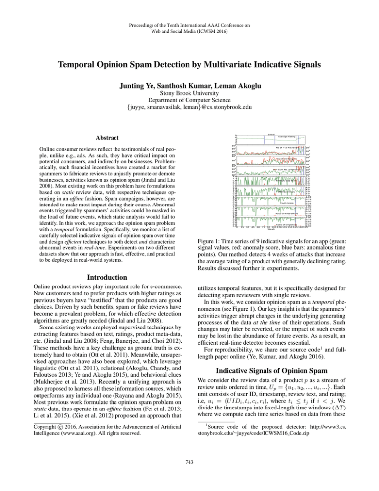
Figure 1: Time series of 9 indicative signals for an app (green:
signal values, red: anomaly score, blue bars: anomalous time
points). Our method detects 4 weeks of attacks that increase
the average rating of a product with generally declining rating.
Results discussed further in experiments.
Introduction
Online product reviews play important role for e-commerce.
New customers tend to prefer products with higher ratings as
previous buyers have “testified” that the products are good
choices. Driven by such benefits, spam or fake reviews have
become a prevalent problem, for which effective detection
algorithms are greatly needed (Jindal and Liu 2008).
Some existing works employed supervised techniques by
extracting features based on text, ratings, product meta-data,
etc. (Jindal and Liu 2008; Feng, Banerjee, and Choi 2012).
These methods have a key challenge as ground truth is extremely hard to obtain (Ott et al. 2011). Meanwhile, unsupervised approaches have also been explored, which leverage
linguistic (Ott et al. 2011), relational (Akoglu, Chandy, and
Faloutsos 2013; Ye and Akoglu 2015), and behavioral clues
(Mukherjee et al. 2013). Recently a unifying approach is
also proposed to harness all these information sources, which
outperforms any individual one (Rayana and Akoglu 2015).
Most previous work formulate the opinion spam problem on
static data, thus operate in an offline fashion (Fei et al. 2013;
Li et al. 2015). (Xie et al. 2012) proposed an approach that
We consider the review data of a product p as a stream of
review units ordered in time, Up = {u1 , u2 , ..., ui , ...}. Each
unit consists of user ID, timestamp, review text, and rating;
i.e, ui = (U IDi , ti , ci , ri ), where ti ≤ tj if i < j. We
divide the timestamps into fixed-length time windows (ΔT )
where we compute each time series based on data from these
c 2016, Association for the Advancement of Artificial
Copyright Intelligence (www.aaai.org). All rights reserved.
1
Source code of the proposed detector: http://www3.cs.
stonybrook.edu/∼juyye/code/ICWSM16 Code.zip
utilizes temporal features, but it is specifically designed for
detecting spam reviewers with single reviews.
In this work, we consider opinion spam as a temporal phenomenon (see Figure 1). Our key insight is that the spammers’
activities trigger abrupt changes in the underlying generating
processes of the data at the time of their operations. Such
changes may later be reverted, or the impact of such events
may be lost in the abundance of future events. As a result, an
efficient real-time detector becomes essential.
For reproducibility, we share our source code1 and fulllength paper online (Ye, Kumar, and Akoglu 2016).
Indicative Signals of Opinion Spam
743
intervals. We identify eight types of indicative signals, and
extract their time series for each product p.
1. Average Rating: This time series tracks the evolution of
cumulative average rating. Let Ūpt = {uk |tk ∈ [0, t∗ΔT )}
denote the set of p’s reviews until the
of time window
end
m
1
t, where |Ūpt | = m. Then, Rpt = m
k=1 rk .
2. Number of Reviews: This time series tracks the total
number of reviews within each time interval. Let Upt =
{uk |tk ∈ [(t−1)∗ΔT, t∗ΔT
)} denote p’s reviews within
window t. Then, Cpt = Upt .
3. Number of Positive/Negative Reviews: We also track the
positive and negative review
counts, as fake reviews have
skewed ratings. +Cpt = {uk |uk ∈ Upt , rk ∈ {4, 5}},
−Cpt = {uk |uk ∈ Upt , rk ∈ {1, 2}}.
4. Rating Entropy: We monitor rating entropy over time.
Let ptr denote the fraction of reviews with rating value
5
equal to r in window t. Then, Ept = − r=1 ptr · log ptr .
5. Ratio of Singletons: We track the ratio of one-time reviewers since fake reviews could be posted by newly created
|U t |
accounts. Spt = Cst , where Ust is the user set who posted
p
their only review (to p) during window t.
6. Ratio of First-timers: Spammers also may target multiple
products simultaneously. Let Uft be the set of p’s reviewers who posted their first but not necessarily only review
during window t, then Fpt =
|Uft |
Cpt
For anomaly detection on the lead time series, one can
use any detection algorithm that provides real-time capability. One important issue is the semantics of the lead signal.
Average rating is cumulative, and our goal is to find change
points in both directions (either increase or decrease). For
this lead, we use the cumulative sum (CUSUM) change detection algorithm (Page 1954). On the other hand, we track the
non-cumulative number of positive and negative reviews per
time window ΔT , with a goal to spot anomalies in the form
of bursts (i.e., large increases). For such leads, we use the
autoregressive (AR) model for modeling the lead series, and
use the deviation from the forecasted value as the anomaly
score s at a new time point.
For change/anomaly detection, choice of a threshold is
critical to flag alerts. For a given (lead) signal and a detector,
we maintain the distribution D(S|T, P ) of the anomalousness
scores S; (i) across time points T and (ii) across products P .
We then employ Cantelli’s inequality2 to identify a theoretical
threshold δ = (D, η), where η is the expected percentage of
anomalies. For a given score stp for product p at time t, we
flag an alert if stp > δ and the anomaly is in the direction
of what a suspicious activity would create (i.e., increase or
decrease in the corresponding signal).
Anomalies in the Supporting Signals
Lead signal alone is not sufficient to indicate the occurrence
of spamming activities. Therefore, we investigate further the
supporting signals, to verify if “alarms” triggered by the lead
signal are indeed the consequences of spamming activities.
In order to detect anomalies in each supporting signal,
we propose L OCAL AR, which only focuses on and scores
the time points around the “alarms” produced by the lead
signal, and hence selectively ignores the other time points.
This reduces the time complexity to sublinear, in terms of the
total number of time points. In the following, we elaborate
on the steps of L OCAL AR, which is shown in Algorithm 1.
At time ti , we check if there is a close-by “alarm” ta in the
lead signal. If not, then we exit the algorithm (Lines 3-4). This
step accelerates the algorithm significantly in two aspects:
(i) it skips anomaly score computation for points away from
the lead “alarms”, as a result of which (ii) feature extraction
for a large body of time points in supporting signals can
also be skipped. Next, we select a proper (integer) k that
minimizes the total square error over a window of L values3
before vi (Lines 5-12). Specifically, we pick a candidate k and initialize the square error sum Sk to 0. We compute the
square error si−j between the inputs vi−j and predictions
v̂i−j of an AR model of order k , for all L values before vi .
Sum of square errors is denoted by Sk . We then choose the
k with the minimum Sk as the order of our AR model at
time ti . As temporal dependence drops by distance in time,
we focus on small k ∈ [1, 5]. Through Lines 13-18, we
carefully examine the time points around ta . We compute the
.
7. Youth Score: We compute the age of the reviewer U IDk
IDk
at the time they posted uk for p, by Ak = tk − tU
,
0
U IDk
where t0
is the time at which reviewer U IDk posted
their first review. The youth score is the average of reviewer ages at the time they posted for p, i.e. Ypt =
1
1
uk ∈U t 2 · (1 − 1+exp (−Ak ) ).
Ct
p
p
8. Temporal Gap Entropy: This series tracks the time-gap
between consecutive reviews {uk , uk+1 } ∈ Upt of p within
window t, creates a histogram, and computes the entropy.
log ΔT +1 t
Gtp = − b=1 2
pb · log ptb , where ptb is the fraction
of gaps in logarithmically-growing bin b in t.
Temporal Opinion Spam Detection
Our temporal approach to opinion spam detection consists
of four main steps: (i) extracting temporal signal values as
defined in the previous section; (ii) detecting changes in what
is called the lead signal; (iii) checking whether we also observe temporal anomalies in the supporting signals; and (iv)
ranking targeted products based on the number and magnitude of anomalies found in their timeline. In the following
subsections, we present the details of steps (ii)-(iv).
Anomalies in the Lead Signal
Of all the indicative signals extracted over time, we dedicate
one of them as the lead signal. The lead can be chosen as
the measure that spammers particularly aim to manipulate
(e.g., avg. rating), or a measure for which spamming activities
could trigger a change (e.g., positive review count).
2
Unlike the t-test which assumes Gaussian data, Cantelli’s inequality does not make any distributional assumptions on D.
3
Window size L is essentially the training data size used to
estimate k. Choice of L poses a trade-off between the estimation
quality and running time. In experiments we find L = 8 effective.
744
Algorithm 1: L OCAL AR
1
2
3
4
5
6
7
8
9
10
11
12
13
14
15
16
17
18
i
Input: ti , ta , L, vi−L−5
,δ
i
Output: sta −2 , Otia −2
if ti − ta > 2 then // exit if no recent anomaly in lead signal
Exit
foreach k ∈ [1, 5] do // select k that minimizes square error
Init Sk = 0
foreach j ∈ [1, L] do
i−j−1
θ = AR(vi−j−k
, k ) (where θ = {ω, μ, σ})
i−j−1
v̂i−j = ω(vi−j−k − μ) + μ
si−j = (vi−j − v̂i−j )2
Sk = Sk + si−j
Figure 2: Stacked bars show daily review counts for 4 detected campaigns in Figure 1 (week before, during, and after
campaign, separated by vertical bars). Stacks represent counts
for ratings 1-5. Notice that spam campaigns involve mostly
5-star reviews (hence the bumpy increase in average rating
week by week after each campaign).
k = kmin
, where ∀k ∈ [1, 5], Sk ≥ Skmin
foreach tj ∈ [ta − 2, ti ] do // check time points around ta
j−1
θj = AR(vj−k
, k)
j−1
v̂j = ωj (vj−k − μj ) + μj
sj = (vj − v̂j )2
if sj > δ & SemSus(vj ) is T rue then
Oj = 1
Experiments
Datasets
SoftWare Marketplace (SWM) consists of reviews for all
software products (apps) from the entertainment category in
a popular online software marketplace. It contains 15,094
apps with over 1.1 million reviews by over 966,000 users,
and spans 198 weeks between July 2008 and April 2012.
F LIPKART contains reviews from flipkart.com, an ecommerce site which provides a platform for sellers to market
products to customers. It contains about 545,000 products
with roughly 3.3 million reviews by 1.1 million users, and
spans 180 weeks between August 2011 to January 2015.
square error for values at and before vi at this step, using the
estimated k. If the square error is larger than the anomaly
threshold and SemSus(vj ) returns T rue4 , then output value
Oj is assigned as 1, i.e. anomalous.
Scoring and Ranking Products
We propose a function to score products by suspiciousness
based on (i) the number and (ii) magnitude of the temporal
anomalies among its indicative signals. Four measures are
designed to quantify product suspiciousness.
First is the fraction of anomalies among product pi ’s 9
9
(l)
indicative signals at tj . That is, f1 (pi , tj ) = l=1 Oj,pi /9,
Results
We manually inspect the top-ranked products from both
datasets, and provide evidence through case studies.
SWM Case I: Game app This app (see Figure 1), which
started off with an average rating of 4, declined below 3-stars
between weeks 75 to 165. A series of spam campaigns are
then executed in weeks 168, 175, 182, and 189 (notice how
these campaigns are organized every 7 weeks—a strong indication of manipulation). When we use ‘Average Rating’
as the lead signal, we spot the first two campaigns, whereas
when ‘Num. of + Reviews’ is used as the lead, all 4 weeks
are detected. Nearly all the supporting signals also change
simultaneously. Figure 2 shows the daily review counts for
the week before, at, and after the spam campaigns, for each
of the 4 detected campaigns, along with the distribution of
ratings per day. Most reviews are from singletons that rated
this app with 4 or 5 stars. We also find that singleton reviews
have duplicates or near duplicates. For example all the following text snippets appear multiple times across different
reviews of this app: “Great app for gamers”, “Great App For
Gaming news”, “Easy to use”, “Must have app for gamers”.
(l)
where Oj,pi ∈ {0, 1} is the anomaly label of signal l of
product pi at tj . The second and third measures are respectively the average and maximum magnitude of the anomalies,
9
9
(l)
(l)
and can be written as f2 (pi , tj ) = l=1 sj,pi / l=1 Oj,pi
(l)
(l)
and f3 (pi , tj ) = maxl=1...9 sj,pi , where sj,pi is the anomaly
score of signal l of product pi at tj . Finally, f4 (pi , tj ) =
9
(l)
l=1 wl · sj,pi is the weighted sum of the anomaly scores,
j
(l)
where wl = 1/ t=1 Ot,pi which is inversely proportional
to the number of anomalies in signal l.
We then use the empirical CDF to normalize the feature
values, i.e. Fg (pi , tj ) = P (fg ≤ fg (pi , tj )), g = 1, . . . , 4,
where Fg (pi , tj ) is the fraction of fg ’s that are smaller than
or equal to fg (pi , tj ) across all products and all time points
before tj . The larger the Fg (pi , tj ), the larger the anomalousness. Finally, we compute pi ’s suspiciousness score A(pi , tj )
at time tj as an average of the Fg (pi , tj )’s.
F LIPKART Case I This product is detected as anomalous
in week 35 (Figure 3 left). During this period, over 80 reviews
are written. Most reviews are rated 3- or 4-stars, but only a
few 5-stars, while being able to increase average rating. These
mixed ratings appear to be for better camouflage. Moreover,
most reviewers are non-singletons (unlike in SWM) although
4
vj is “semantically suspicious” (denoted as SemSus(vj ) =
T rue) if either (i) vj > vj−1 and large value indicates spamming
activities (e.g., ratio of singletons), or (ii) if vj < vj−1 and small
value indicates suspicious behaviors (e.g., rating entropy).
745
Figure 4: Series for 3 lead signals for a F LIPKART book.
(i) monitors a comprehensive list of indicative signals of spam
over time, (ii) spots anomalous events in real-time, and (iii)
provides pointers to specific time intervals for manual inspection and characterization. As such, our approach exhibits
desirable properties, as it is online, efficient, and descriptive.
Importantly, our method is general enough to be employed
for other applications in which multiple signals are monitored over time, such as enterprise security, environmental
monitoring, and surveillance systems.
Acknowledgments. Research is supported by the NSF
CAREER 1452425, IIS 1408287, the DARPA Transparent
Computing Program under Contract No. FA8650-15-C-7561,
a Facebook Faculty Gift, and an R&D grant from Northrop
Grumman. Any conclusions expressed in this material are of
the authors and do not necessarily reflect the views, expressed
or implied, of the funding parties
Figure 3: Partial time series for 9 indicative signals for two
different products from F LIPKART that were spammed by
same reviewers during same time periods (week 35 and 40).
they are young accounts. This suggests that other products
might also have been spammed by the same reviewers. We
confirmed this conjecture by finding that a list of other products (one of which is shown in Figure 3 right) are rated similarly by these same users during the same time period (these
periods are also detected as anomalous by our method). Further, we find that all these products are hair-related, including
straighteners, dryers, and shavers, potentially belonging to
the same seller.
References
Akoglu, L.; Chandy, R.; and Faloutsos, C. 2013. Opinion fraud
detection in online reviews by network effects. In ICWSM.
Fei, G.; Mukherjee, A.; Liu, B.; Hsu, M.; Castellanos, M.; and
Ghosh, R. 2013. Exploiting burstiness in reviews for review spammer detection. In ICWSM.
Feng, S.; Banerjee, R.; and Choi, Y. 2012. Syntactic stylometry for
deception detection. In ACL.
Jindal, N., and Liu, B. 2008. Opinion spam and analysis. In WSDM.
Li, H.; Chen, Z.; Mukherjee, A.; Liu, B.; and Shao, J. 2015. Analyzing and detecting opinion spam on a large-scale dataset via temporal
and spatial patterns. In ICWSM.
Mukherjee, A.; Kumar, A.; Liu, B.; Wang, J.; Hsu, M.; Castellanos,
M.; and Ghosh, R. 2013. Spotting opinion spammers using behavioral footprints. In KDD.
Ott, M.; Choi, Y.; Cardie, C.; and Hancock, J. T. 2011. Finding
deceptive opinion spam by any stretch of the imagination. In ACL.
Page, E. S. 1954. Continuous Inspection Schemes. Biometrika 41.
Rayana, S., and Akoglu, L. 2015. Collective opinion spam detection:
Bridging review networks and metadata. In KDD.
Xie, S.; Wang, G.; Lin, S.; and Yu, P. S. 2012. Review spam
detection via temporal pattern discovery. In KDD.
Ye, J., and Akoglu, L. 2015. Discovering opinion spammer groups
by network footprints. In ECML/PKDD.
Ye, J.; Kumar, S.; and Akoglu, L.
2016.
Temporal
Opinion Spam Detection by Multivariate Indicative Signals.
http://arxiv.org/abs/1603.01929.
F LIPKART Case II Our second case study from F LIP KART is for an anomalous book, whose average rating increased to 4.4 on week 95 (see Figure 4). We find that this
book received 125 5-star reviews in mainly two days during
that week. Surprisingly those were from non-singletons, who
also reviewed another product—also a book (!) Further investigation revealed that those were 2 out of 3 books of an author.
Both books have average ratings ∼4.4, while they are rated
∼3.3 on another review system, Goodreads.com. Moreover, we
found that almost all 125 reviewers have similar behavioral
pattern: 5-star reviews written 7 PM–11PM on June 8 and
11AM–7PM on June 9, 2013. What is more, their reviews
follow nearly the same order for both books.
For more details on these case studies as well as additional
ones, we refer to (Ye, Kumar, and Akoglu 2016).
Conclusion
Opinion spam has become a prevalent problem, for which
a vast body of methods operate in an offline fashion on a
collection of static data. In this work, we brought emphasis to
the aspect of time, and approached this problem with a novel
temporal formulation. We proposed a new methodology that
746