Proceedings of the Thirtieth AAAI Conference on Artificial Intelligence (AAAI-16)
Approximate K-Means++ in Sublinear Time
Olivier Bachem
Mario Lucic
S. Hamed Hassani
Andreas Krause
ETH Zurich
olivier.bachem@inf.ethz.ch
ETH Zurich
lucic@inf.ethz.ch
ETH Zurich
hamed@inf.ethz.ch
ETH Zurich
krausea@ethz.ch
k-means++. In the seeding step of k-means++, the cluster centers are sampled iteratively using D2 -sampling: First,
a cluster center is chosen uniformly at random from the data
points. Then, in each of k iterations, a data point is selected
as a new cluster center with probability proportional to its
distance to the already sampled cluster centers. Even without
assumptions on the data, the resulting solution is in expectation O(log k)-competitive with regards to the optimal solution (Arthur and Vassilvitskii, 2007). While k-means++
is easy to implement, it is non-trivial to apply it to large
problems. k-means++ has to make a full pass through
the data for every cluster center sampled. This leads to a
complexity of Θ(nkd) where n is the number of data points,
k the number of cluster centers and d the dimensionality of
the data. Even if k is moderate, this can be computationally
infeasible for massive datasets. This motivates our search
for a seeding method with a lower, potentially even sublinear, complexity in the number of data points that retains
both the empirical and theoretical benefits of k-means++.
Abstract
The quality of K-Means clustering is extremely sensitive to proper initialization. The classic remedy is
to apply k-means++ to obtain an initial set of centers that is provably competitive with the optimal solution. Unfortunately, k-means++ requires k full passes
over the data which limits its applicability to massive
datasets. We address this problem by proposing a simple and efficient seeding algorithm for K-Means clustering. The main idea is to replace the exact D2 -sampling
step in k-means++ with a substantially faster approximation based on Markov Chain Monte Carlo sampling. We prove that, under natural assumptions on the
data, the proposed algorithm retains the full theoretical guarantees of k-means++ while its computational
complexity is only sublinear in the number of data
points. For such datasets, one can thus obtain a provably good clustering in sublinear time. Extensive experiments confirm that the proposed method is competitive with k-means++ on a variety of real-world, largescale datasets while offering a reduction in runtime of
several orders of magnitude.
1
But is it even worth pursuing a fast seeding algorithm?
After all, both evaluating the quality of such a seeding and
running one iteration of Lloyd’s algorithm exhibit the same
Θ(nkd) complexity as the seeding step of k-means++.
Hence, one might argue that there is no benefit in reducing
the complexity of the k-means++ seeding step as it is
dominated by these two other operations. There are two
shortcomings to this argument: Firstly, k-means++ is an
inherently sequential algorithm of k dependent iterations
and, as such, difficult to parallelize in a distributed setting.
Evaluating the quality of a K-Means solution, however,
can be done in parallel using a single MapReduce step.
Similarly, Lloyd’s algorithm can also be implemented in
MapReduce (Zhao, Ma, and He, 2009). Secondly, there
are many use cases where one requires fast seeding without
evaluating the quality of the seeding or running Lloyd’s
algorithm subsequently. For example, the quality of such
a solution can be improved using fast algorithms such as
online (Bottou and Bengio, 1994) or mini-batch K-Means
(Sculley, 2010) which may be run for less than O(n) iterations in practice. Furthermore, various theoretical results
such as coreset constructions (Bachem, Lucic, and Krause,
2015) rely on the theoretical guarantee of k-means++.
Hence, a fast seeding algorithm with a strong theoretical
guarantee would have an impact on all these applications.
Introduction
The goal of K-Means clustering is to find a set of k cluster
centers for a dataset such that the sum of squared distances
of each point to its closest cluster center is minimized. It is
one of the classic clustering problems and has been studied for several decades. Yet even today, it remains a relevant
problem: Lloyd’s algorithm (Lloyd, 1982), a local search algorithm for K-Means, is still one of the ten most popular
algorithms for data mining according to Wu et al. (2008)
and is implemented as a standard clustering method in most
machine learning libraries. In the last few years, K-Means
clustering has further been studied in various fields of machine learning such as representation learning (Coates, Lee,
and Ng, 2011; Coates and Ng, 2012) and Bayesian nonparametrics (Kulis and Jordan, 2012).
It is well-known that K-Means clustering is highly sensitive to proper initialization. The classical remedy is to use
a seeding procedure proposed by Arthur and Vassilvitskii
(2007) that together with Lloyd’s algorithm is known as
c 2016, Association for the Advancement of Artificial
Copyright Intelligence (www.aaai.org). All rights reserved.
1459
Our Contributions. In this paper, we propose a simple, but novel algorithm based on Markov Chain Monte
Carlo (MCMC) sampling to quickly obtain a seeding for
the K-Means clustering problem. The algorithm can be run
with varying computational complexity and approximates
the seeding step of k-means++ with arbitrary precision
as its complexity is increased. Furthermore, we show that
for a wide class of non-pathological datasets convergence is
fast. Under these mild and natural assumptions, it is sufficient to run our algorithm with complexity sublinear in the
number of data points to retain the same O(log k) guarantee
as k-means++. This implies that for such datasets, a provably good K-Means clustering can be obtained in sublinear
time. We extensively evaluate the proposed algorithm empirically and compare it to k-means++ as well as two other
approaches on a variety of datasets.
2
were considered in the original paper (Arthur and Vassilvitskii, 2007) as well as in Brunsch and Röglin (2011). A polynomial time approximation scheme for K-Means using D 2 sampling was proposed in Jaiswal, Kumar, and Sen (2014)
and Jaiswal, Kumar, and Yadav (2015).
Several ideas extending k-means++ to the streaming
setting were explored: A single-pass streaming algorithm
based on coresets and k-means++ was proposed in Ackermann et al. (2012). The main drawback of this approach
is that the size of the coreset is exponential in the dimensionality of the data. Ailon, Jaiswal, and Monteleoni (2009)
suggest a streaming algorithm based on Guha et al. (2003)
that provides the same O(log k) guarantee as k-means++
with a complexity of O(ndk log n log k).
Bahmani et al. (2012) propose a parallel version of
k-means++ called k-means that obtains the same
O(log k) guarantee with a complexity of Θ(ndk log n). The
main idea is to replace the k sequential sampling rounds of
k-means++ by r = Θ(log n) rounds in each of which
l = Θ(k) points are sampled in parallel. In a final step,
the Θ(k log n) sampled points are clustered again using
k-means++ to produce a final seeding of k points. As
a result, the computational complexity of k-means is
higher than k-means++ but can be efficiently distributed
across different machines. In Section 6, we will compare
k-means with our proposed method on various datasets.
Background & Related Work
K-Means clustering. Let X denote a set of n points in Rd .
The K-Means clustering problem is to find a set C of k cluster centers in Rd such that the quantization error φC (X ) is
minimized, where
d(x, C)2 =
minx − c22 .
φC (X ) =
x∈X
x∈X
c∈C
In this paper, we implicitly use the Euclidean distance function; however, any distance function d(x, x ) may be used.
The optimal quantization error is denoted by φkOP T (X ).
k-means++ seeding. The seeding step of k-means++
(Arthur and Vassilvitskii 2007) works by sampling an initial
cluster center uniformly at random and then adaptively sampling (k − 1) additional cluster centers using D2 -sampling.
More specifically, in each iteration i = 2, . . . , k, the data
point x ∈ X is added to the set of already sampled cluster
centers Ci−1 with probability
p(x) = d(x, Ci−1 )2
.
2
x ∈X d(x , Ci−1 )
3
Approximate D2 -sampling
In each iteration of D2 -sampling, the k-means++ algorithm has a computational complexity of Θ(nd) as it needs
to calculate the sampling probabilities p(x) in (1) for every data point. We aim to reduce the complexity by approximating the D2 -sampling step: we strive for a fast sampling
scheme whose implied sampling probabilities p̃(x) are close
to p(x). To formalize this notion of closeness, we use the total variation distance which measures the maximum difference in probabilities that two distributions assign to an event.
More formally, let Ω be a finite sample space on which two
probability distributions p and q are defined. The total variation distance between p and q is given by
1
|p(x) − q(x)|.
(2)
p − qTV =
2
(1)
The algorithm’s time complexity is Θ(nkd) and the resulting seeding Ck is in expectation O(log k) competitive with
respect to the optimal quantization error φkOP T (X ) (Arthur
and Vassilvitskii, 2007), i.e.
x∈Ω
In Section 5 we will show that using total variation distance
we can bound the solution quality obtained by our algorithm. Informally, if the total variation distance is less than
, we are able to to retain the same theoretical guarantees as
k-means++ with probability at least (1 − ).
MCMC approximation. The Metropolis-Hastings algorithm (Hastings 1970) (with an independent, uniform proposal distribution) applied to a single step of D2 -sampling
works as follows: We uniformly sample an initial state x0
from the point set X and then iteratively build a Markov
chain. In each iteration j, we uniformly sample a candidate
point yj and calculate the acceptance probability
d(yj , C)2
p(yj )
= min 1,
. (3)
π = min 1,
p(xj−1 )
d(xj−1 , C)2
E [φCk (X )] ≤ 8(log2 k + 2)φkOP T (X ).
Related work. Previously, the same idea as in
k-means++ was explored in Ostrovsky et al. (2006) where
it was shown that, under some data separability assumptions, the algorithm provides a constant factor approximation. Similar assumptions were analyzed in Balcan, Blum,
and Gupta (2009), Braverman et al. (2011), Shindler, Wong,
and Meyerson (2011), Jaiswal and Garg (2012) and Agarwal, Jaiswal, and Pal (2013). Without any assumption on the
data, it was shown that D2 -sampling leads to a constant factor approximation if Ω(k log k) (Ailon, Jaiswal, and Monteleoni, 2009) or Ω(k) (Aggarwal, Deshpande, and Kannan,
2009) centers are sampled. Bad instances for k-means++
1460
With probability π we then set the state xj to yj and with
probability 1 − π to xj−1 . For a Markov chain of total length
m, we only need to calculate the distance between m data
points and the cluster centers since the normalization constants of p(yj ) and p(xj−1 ) in (3) cancel. By design, the
stationary distribution of this Markov chain is the target distribution p(x). This implies that the distribution p̃m (x) of
the m-th state xm converges to p(x) as m → ∞. Furthermore, the total variation distance decreases at a geometric
rate with respect to the chain length m (Cai, 2000) as
m 1
p̃m − pTV = O
1−
γ
where
(4)
γ = n max p(x).
x∈X
This implies that there is a chain length m = O γ log 1
that achieves a total variation distance of at most . Intuitively, γ measures the difficulty of approximately sampling
from p(x) and depends on the current set of centers C and
the dataset X . We remark that the total variation distance increases with γ. For now, we assume γ to be given and defer
the detailed analysis to Section 5.
4
Theorem 1. Let k > 0 and 0 < < 1. Let p++ (C) be
the probability of sampling a seeding C using k-means++
and pmcmc (C) the probability using K - MC2 (Algorithm 1).
Then,
pmcmc − p++ TV ≤ for a chain length m = O γ log k where
d(x, C)2
.
2
C⊂X ,|C|≤k x∈X
x ∈X d(x , C)
The resulting complexity of Algorithm 1 is O γ k 2 d log k .
The proof is given in Section B of the Appendix. This result implies that we can use K - MC2 to approximate the seeding step of k-means++ to arbitrary precision. The required
chain length m depends linearly on γ which is a uniform
upper bound on γ for all possible sets of centers C. In the
next section, we provide a detailed analysis of γ and quantify its impact on the quality of seeding produced by K - MC2 .
γ =
max n max
5
Analysis
In the previous section, we saw that the rate of convergence
of K - MC2 depends linearly on γ . By definition, γ is trivially
bounded by n and it is easy to construct a dataset achieving
this bound: Consider the 2-Means clustering problem and
let (n − 1) points be in an arbitrarily small cluster while
a single point lies at some distance away. With probability
(1 − n1 ), a point from the first group is sampled as the initial cluster center. In the subsequent D2 -sampling step, we
are thus required to sample the single point with probability approaching one. For such a pathological dataset, it is
impossible to approximate D2 -sampling in sublinear time.
Our proposed algorithm is consistent with this result as it
would require linear complexity with regards to the number
of data points for this dataset. Fortunately, such pathological
datasets rarely occur in a practical setting. In fact, under very
mild and natural assumptions on the dataset, we will show
that γ is at most sublinear in the number of data points.
To this end, we assume that the dataset X is sampled i.i.d.
from a base distribution F and note that γ can be bounded
by two terms α and β, i.e.
maxx∈X d(x, μ(X ))2 φ1OP T (X )
γ ≤ 4 1 (5)
k
2
x ∈X d(x , μ(X )) φOP T (X )
n
Approximate K-Means++ using K - MC2
It is straightforward to extend this MCMC-based sampler to
approximate the full seeding step of k-means++: We first
sample an initial cluster center uniformly at random. Then,
for each of the remaining k − 1 iterations, we build an independent Markov chain of length m and use the last element
as the new cluster center. We call this algorithm K - MC2 and
provide pseudo-code in Algorithm
1. The complexity of the
proposed algorithm is Θ mk 2 d . In particular, it does not
depend on the number of data points n.
Theorem 1 guarantees convergence of Algorithm 1 to
k-means++ in terms of total variation distance. Since the
(k − 1) Markov chains are independent, we may use a union
bound: If the sampling induced by each chain has a total
variation distance of at most /(k − 1), then the total variation distance between the sampling induced by K - MC2 and
the sampling induced by k-means++ is at most (as shown
in the proof of Theorem 1).
α
Algorithm 1 K - MC2
β
denotes
where μ(X ) denotes the mean of X and
the quantization error of the optimal solution of k centers
(see Section C of the Appendix for a proof).
Tail behavior of distribution F . The first term α measures the ratio between the maximum and the average of the
squared distances between the data points and their empirical mean. In the pathological example introduced above, α
would approach (n − 1). Yet, under the following assumption, α grows sublinearly in n as formally stated and proven
in Section A.1 of the Appendix.
(A1) For distributions F with finite variance and exponential tails1 , α is independent of k and d and w.h.p.
α = O log2 n .
φkOP T (X )
Require: Dataset X , number of centers k, chain length m
c1 ← point uniformly sampled from X
C1 ← {c1 }
for i = 2, 3, . . . , k do
x ← point uniformly sampled from X
dx ← d(x, Ci−1 )2
for j = 2, 3, . . . , m do
y ← point uniformly sampled from X
dy ← d(y, Ci−1 )2
d
if dxy > Unif(0, 1) then
x ← y, dx ← dy
Ci ← Ci−1 ∪ {x}
return Ck
1
1461
∃c, t such that P [d(x, μ(F )) > a] ≤ ce−at where x ∼ F .
Table 1: Datasets with size n, dimensionality d and estimated values for α and β
This assumption is satisfied by the univariate and multivariate Gaussian as well as the Exponential and Laplace distributions, but not by heavy tailed distributions such as the
Pareto distribution. Furthermore, if α is sublinear in n for
all components of a mixture, then α is also sublinear for
the mixture itself. For distributions with finite variance and
bounded support, we even show a bound on α that is independent of n.
Nondegeneracy of distribution F . The second term β
measures the reduction in quantization error if k centers are
used instead of just one. Without prior assumptions β can be
unbounded: If a dataset consists of at most k distinct points,
the denominator of the second term in (5) is zero. Yet, what
is the point of clustering such a dataset in practice if the
solution is trivial? It is thus natural to assume that F is nondegenerate, i.e., its support is larger than k. Furthermore, we
expect β to be independent of n if n is sufficiently large: Due
to the strong consistency of K-Means the optimal solution on
a finite sample converges to the optimal quantizer of the generating distribution as n → ∞ (Pollard, 1981) and such an
optimal quantizer is by definition independent of n. At the
same time, β should be non-increasing with respect to k as
additional available cluster centers can only reduce the optimal quantization error. This allows us to derive a very general result (formally stated and proven in Section A.2 of the
Appendix) that for distributions F that are “approximately
uniform” on a hypersphere, β is independent of n.
(A2) For distributions F whose minimal and maximal density on a hypersphere with nonzero probability mass is
bounded by a constant, β is independent of n and w.h.p.
N
D
α
β̃ ( K =200)
80000
145751
59209
45811883
11620300
515345
17
74
3
5
57
90
546.27
1267.65
2.68
2.33
7.82
525.67
3.04
1.81
51.67
57.09
14.17
1.23
DATASET
CSN
KDD
USGS
WEB
BIGX
SONG
The proof is provided in Section C of the Appendix. The
significance of this result is that, under natural assumptions,
it is sufficient to run K - MC2 with complexity sublinear in the
number of data points to retain the theoretical guarantee of
k-means++. Hence, one can obtain a provably good clustering for K-Means in sublinear time for such datasets.
6
Experiments
Datasets. We use six different datasets: USGS (United States
Geological Survey, 2010), CSN (Faulkner et al., 2011), KDD
(KDD Cup, 2004), BIGX (Ackermann et al., 2012), WEB
(Yahoo! Labs, 2008) and SONG (Bertin-Mahieux et al.,
2011). Table 1 shows the size and number of dimensions
of these datasets as well as estimates of both α and β. We
directly calculate α using (5) and approximate β by replacing the optimal solution φkOP T (X ) in (5) with the solution
obtained using k-means++.
Methods. We compare the algorithm K - MC2 to four alternative methods (k-means++, RANDOM, HEURISTIC and
k-means). We run K - MC2 with different chain lengths,
i.e. m ∈ {1, 2, 5, 10, 20, 50, 100, 150, 200}. As the main
baselines, we consider the seeding step of k-means++
as well as RANDOM, a seeding procedure that uniformly
samples k data points as cluster centers. We further propose the following HEURISTIC: It works by uniformly
sampling s points and then running the seeding step
of k-means++ on this subset. Similar to K - MC2 , we
set s ∈ {100, 200, 500, . . . , 10 000, 15 000, 20 000}. Finally, we also compare to k-means. We use r = 5
rounds and a variety of oversampling factors, i.e. l ∈
{0.02k, 0.05k, 0.1k, 0.2k, 0.5k, 1k, 2k}.
Experimental setup. For the datasets USGS, CSN and
KDD , we set k = 200 and train all methods on the full
datasets. We measure the number of distance evaluations
and the quality of the solution found in terms of quantization error on the full dataset. For the datasets BIGX, WEB
and SONG, we set k = 2000 and train on all but 250 000
points which we use as a holdout set for evaluation. We consider both training error and holdout error for the following
reason: On one hand, the theoretical guarantees for both K MC 2 and k-means++ hold in terms of training error. On
the other hand, in practice, one is usually interested in the
generalization error.
As all the considered methods are randomized procedures, we run them repeatedly with different initial random
seeds. We average the obtained quantization errors and use
β = O(k).
This property holds for a wide family of continuous probability distribution functions including the univariate and
multivariate Gaussian, the Exponential and the Laplace distribution. Again, if β is bounded for all components of a
mixture, then β is also bounded for the mixture.
Solution quality of K - MC2 . These two assumptions do
not only allow us to bound γ and thus obtain favourable
convergence, but also to analyze the quality of solutions generated by K - MC2 . In particular, we show in Section C of the
Appendix that the expected quantization error φK - MC2 of Algorithm 1 is bounded by
E [φK - MC2 ] ≤ E [φk-means++ ] + 2βφkOP T (X ).
Hence, by setting the total variation distance = O(1/β),
the second term becomes a constant factor of φkOP T (X ). By
applying Theorem 1 with m = O(αβ log βk), the solution
sampled from K - MC2 is in expectation O(log k)-competitive
to the optimal solution and we obtain the following theorem.
Theorem
2. Let k > 0 and X be a dataset with α =
O log2 n and β = O(k), i.e. assume (A1) and (A2). Let
C be the set of centers sampled
by K - MC2 (Algorithm 1)
2
with m = O k log n log k . Then we have
E [φC (X )] ≤ O(log k)φkOP T (X ).
The total complexity is O k 3 d log2 n log k .
1462
Table 2: Experimental results.
R ELATIVE ERROR VS . K - MEANS ++
K - MEANS ++
RANDOM
2
(m = 20)
2
K - MC (m = 100)
2
K - MC (m = 200)
K - MC
HEURISTIC
HEURISTIC
HEURISTIC
(s = 2000)
(s = 10000)
(s = 20000)
K - MEANS K - MEANS K - MEANS (r = 5, l = 0.02k)
(r = 5, l = 0.2k)
(r = 5, l = 2k)
S PEEDUP VS . K - MEANS ++ ( DISTANCE EVALUATIONS )
CSN
KDD
USGS
BIGX
WEB
SONG
CSN
KDD
USGS
BIGX
WEB
SONG
0.00%
0.00%
0.00%
0.00%
0.00%
0.00%
1.0×
1.0×
1.0×
1.0×
1.0×
1.0×
394.50%
307.44%
315.50%
11.45%
105.34%
9.74%
-
-
-
-
-
-
63.58%
14.67%
6.53%
32.62%
2.94%
1.00%
2.63%
-0.33%
-0.83%
0.05%
0.13%
-0.03%
0.77%
-0.00%
0.01%
0.38%
-0.02%
-0.02%
40.0×
8.0×
4.0×
72.9×
14.6×
7.3×
29.6×
5.9×
3.0×
568.5×
113.7×
56.9×
2278.1×
455.6×
227.8×
13.3×
2.7×
1.3×
94.72%
29.22%
13.99%
73.28%
9.55%
2.22%
5.56%
0.20%
0.27%
0.38%
0.10%
0.02%
2.12%
0.15%
0.07%
0.69%
0.15%
0.05%
40.0×
8.0×
4.0×
72.9×
14.6×
7.3×
29.6×
5.9×
3.0×
568.5×
113.7×
56.9×
2278.1×
455.6×
227.8×
13.3×
2.7×
1.3×
335.61%
2.12%
-3.75%
118.03%
0.71%
-6.22%
2356.06%
19.13%
-3.78%
223.43%
1.74%
-2.43%
562.23%
11.03%
-2.04%
40.54%
-0.34%
-5.16%
9.6×
1.0×
0.1×
9.0×
1.0×
0.1×
8.9×
1.0×
0.1×
10.0×
1.0×
0.1×
9.5×
1.0×
0.1×
9.8×
1.0×
0.1×
7
the standard error of the mean to construct 95% confidence
intervals. For each method, we further calculate the relative
error and the speedup in terms of distance evaluations with
respect to our main baseline k-means++.
Conclusion
2
We propose K - MC , an algorithm to quickly obtain an initial solution to the K-Means clustering problem. It has several attractive properties: It can be used to approximate the
seeding step of k-means++ to arbitrary precision and, under natural assumptions, it even obtains provably good clusterings in sublinear time. This is confirmed by experiments
on real-world datasets where the quality of produced clusterings is similar to those of k-means++ but the runtime
is drastically reduced. K - MC2 further outperforms a heuristic approach based on subsampling the data and produces
fast but competitive seedings with a computational budget
unattainable by k-means. We posit that our technique can
be extended to improve on other theoretical results for D2 sampling as well as to other clustering problems.
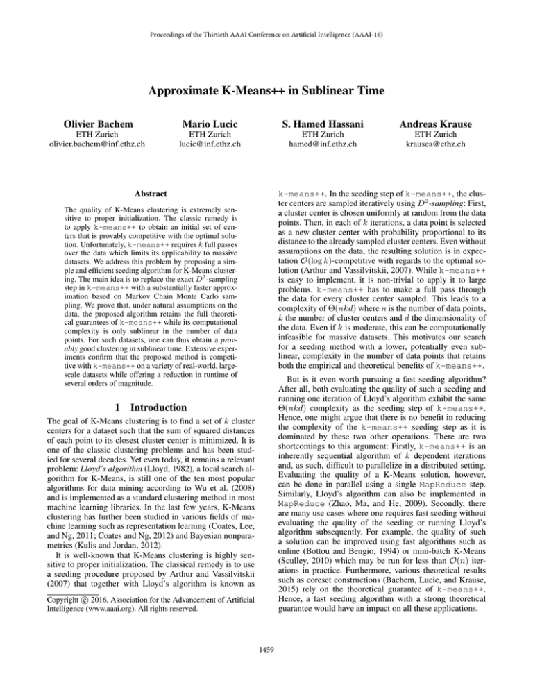
Discussion. The experimental results are displayed in
Figures 1 and 2 and Table 2. As expected, k-means++
produces substantially better solutions than RANDOM (see
Figure 1). For m = 1, K - MC2 essentially returns a uniform
sample of data points and should thus exhibit the same solution quality as RANDOM. This is confirmed by the results in
Figure 1. As the chain length m increases, the performance
of K - MC2 improves and converges to that of k-means++.
Even for small chain lengths, K - MC2 is already competitive
with the full k-means++ algorithm. For example, on BIGX,
K - MC 2 with a chain length of m = 20 exhibits a relative error of only 0.05% compared to k-means++ (see Table 2).
At the same time, K - MC2 is 586.5× faster in terms of distance evaluations.
Acknowledgments. We would like to thank Sebastian
Tschiatschek and the anonymous reviewers for their comments. This research was partially supported by ERC StG
307036 and the Zurich Information Security Center.
K - MC 2 significantly outperforms HEURISTIC on all
datasets (see Figure 1). For the same number of distance
evaluations K - MC2 achieves a smaller quantization error: In
the case of BIGX, HEURISTIC with s = 2000 exhibits a relative error of 0.38% compared to the 0.05% of K - MC2 with
a chain length of m = 20. In contrast to HEURISTIC, K - MC2
further offers the theoretical guarantees presented in Theorems 1 and 2.
References
Ackermann, M. R.; Märtens, M.; Raupach, C.; Swierkot, K.; Lammersen, C.; and Sohler, C. 2012. StreamKM++: A clustering algorithm for data streams. Journal of Experimental Algorithmics
17:2–4.
Figure 2 shows the relationship between the performance
of k-means and the number of distance evaluations. Even
with five rounds, k-means is able to match the performance of the inherently sequential k-means++ and even
outperforms it if more computational effort is invested.
However, as noted in the original paper (Bahmani et al.,
2012), k-means performs poorly if it is run with low computational complexity, i.e. if r · l < k.
Agarwal, M.; Jaiswal, R.; and Pal, A. 2013. k-means++ under
approximation stability. In Theory and Applications of Models of
Computation. Springer. 84–95.
Aggarwal, A.; Deshpande, A.; and Kannan, R. 2009. Adaptive
sampling for k-means clustering. In Approximation, Randomization, and Combinatorial Optimization. Algorithms and Techniques.
Springer. 15–28.
Ailon, N.; Jaiswal, R.; and Monteleoni, C. 2009. Streaming kmeans approximation. In Advances in Neural Information Processing Systems (NIPS), 10–18.
As such, K - MC2 and k-means have different use scenarios: k-means allows one to run the full k-means++
seeding step in a distributed manner on a cluster and potentially obtain even better seedings than k-means++ at the
cost computational effort. In contrast, K - MC2 produces approximate but competitive seedings on a single machine at a
fraction of the computational cost of both k-means++ and
k-means.
Arthur, D., and Vassilvitskii, S. 2007. k-means++: The advantages
of careful seeding. In Symposium on Discrete Algorithms (SODA),
1027–1035. Society for Industrial and Applied Mathematics.
Bachem, O.; Lucic, M.; and Krause, A. 2015. Coresets for nonparametric estimation - the case of DP-means. In International
Conference on Machine Learning (ICML).
1463
CSN (k=200)
×105
5.0
Training error
4.5
k-mc2
heuristic
k-means++
random
m=1
4.0
m=2
3.5
m=5
3.0
m=100
m=200
2.0
1.5
8
m=2
6
m=5
1
106
107
Holdout error
1.32
k-mc2
heuristic
k-means++
random
m=1
1.30
1.28
m=2
1.24
105
2.2
1.22
m=100
m=20
m=200
m=5
3
1.8
m=2
104
0.8
109
105
106
7.3
107
SONG (k=2000)
×1011
7.2
m=5
m=100
m=20
m=200
k-mc2
heuristic
k-means++
random
m=1
7.1
7.0
m=2
6.9
1.2
1.0
108
m=20 m=100
m=200
Distance evaluations
k-mc2
heuristic
k-means++
random
m=1
1.18
107
107
2.0
1.20
106
106
WEB (k=2000)
×102
1.4
m=5
m=2
1
104
1.6
1.26
5
Distance evaluations
BIGX (k=2000)
×1010
k-mc2
heuristic
k-means++
random
m=1
2
Distance evaluations
1.34
6
4
m=100
m=200
3
2
USGS (k=200)
×102
7
m=20
4
0.5
105
m=1
7
1.0
104
k-mc2
heuristic
k-means++
random
5
m=20
2.5
KDD (k=200)
×1011
9
m=5
6.8
m=20
6.7
m=100
m=200
6.6
6.5
106
107
Distance evaluations
108
109
106
Distance evaluations
107
108
109
Distance evaluations
Figure 1: Average quantization error vs. number of distance evaluations for K - MC2 and HEURISTIC as well as the average
quantization error (without the number of distance evaluations) for k-means++ and RANDOM. K - MC2 quickly converges to
full k-means++ and outperforms HEURISTIC. Shaded areas denote 95% confidence intervals.
5.0
CSN (k=200)
×105
9
Training error
4.5
4.0
KDD (k=200)
×1011
8
k-means++
k-mc2
3.5
k-means++
k-mc2
k-means
7
k-means
3.0
k-means
6
2.5
5
2.0
4
1.5
3
1.0
1.0
2
0.5
0.5
1
3.0
2.5
2.0
1.5
105
106
107
108
109
0.0
104
105
Distance evaluations
4.0
×1010
106
107
108
109
104
Distance evaluations
BIGX (k=2000)
7
k-means++
k-mc2
3.5
USGS (k=200)
×103
k-means++
k-mc2
3.5
104
Holdout error
4.0
k-means
k-means
5
3.0
9.5
k-means++
k-mc2
6
106
107
108
109
Distance evaluations
WEB (k=2000)
×102
105
×1011
SONG (k=2000)
k-means++
k-mc2
9.0
k-means
8.5
4
8.0
3
7.5
2.5
2.0
2
7.0
1.5
1
6.5
1.0
0
106
107
108
109
1010
Distance evaluations
1011
1012
6.0
106
107
108
109
1010
Distance evaluations
1011
1012
106
107
108
109
1010
Distance evaluations
Figure 2: Average quantization error vs. number of distance evaluations for K - MC2 , k-means++ and k-means. K - MC2
obtains competitive solutions significantly faster than both k-means++ and k-means.
1464
Pollard, D. 1981. Strong consistency of k-means clustering. The
Annals of Statistics 9(1):135–140.
Sculley, D. 2010. Web-scale k-means clustering. In World Wide
Web Conference (WWW), 1177–1178. ACM.
Shindler, M.; Wong, A.; and Meyerson, A. W. 2011. Fast and
accurate k-means for large datasets. In NIPS, 2375–2383.
United States Geological Survey. 2010. Global Earthquakes
(1.1.1972-19.3.2010). Retrieved from the mldata.org repository.
Wu, X.; Kumar, V.; Ross Quinlan, J.; Ghosh, J.; Yang, Q.; Motoda,
H.; McLachlan, G.; Ng, A.; Liu, B.; Yu, P.; Zhou, Z.-H.; Steinbach,
M.; Hand, D.; and Steinberg, D. 2008. Top 10 algorithms in data
mining. Knowledge and Information Systems 14(1):1–37.
Yahoo! Labs. 2008. R6A - Yahoo! Front Page Today Module User
Click Log Dataset. Retrieved from research.yahoo.com repository.
Zhao, W.; Ma, H.; and He, Q. 2009. Parallel k-means clustering
based on MapReduce. In Cloud Computing. Springer. 674–679.
Bahmani, B.; Moseley, B.; Vattani, A.; Kumar, R.; and Vassilvitskii, S. 2012. Scalable k-means++. Very Large Data Bases (VLDB)
5(7):622–633.
Balcan, M.-F.; Blum, A.; and Gupta, A. 2009. Approximate clustering without the approximation. In Symposium on Discrete Algorithms (SODA), 1068–1077. Society for Industrial and Applied
Mathematics.
Bertin-Mahieux, T.; Ellis, D. P.; Whitman, B.; and Lamere, P. 2011.
The Million Song Dataset. In International Conference on Music
Information Retrieval.
Bottou, L., and Bengio, Y. 1994. Convergence properties of the kmeans algorithms. In Advances in Neural Information Processing
Systems (NIPS), 585–592.
Braverman, V.; Meyerson, A.; Ostrovsky, R.; Roytman, A.;
Shindler, M.; and Tagiku, B. 2011. Streaming k-means on wellclusterable data. In Symposium on Discrete Algorithms (SODA),
26–40. Society for Industrial and Applied Mathematics.
Brunsch, T., and Röglin, H. 2011. A bad instance for k-means++.
In Theory and Applications of Models of Computation. Springer.
344–352.
Cai, H. 2000. Exact bound for the convergence of Metropolis
chains. Stochastic Analysis and Applications 18(1):63–71.
Coates, A., and Ng, A. Y. 2012. Learning feature representations
with k-means. In Neural Networks: Tricks of the Trade. Springer.
561–580.
Coates, A.; Lee, H.; and Ng, A. Y. 2011. An analysis of singlelayer networks in unsupervised feature learning. In International
Conference on Artificial Intelligence and Statistics (AISTATS), volume 1001.
Faulkner, M.; Olson, M.; Chandy, R.; Krause, J.; Chandy, K. M.;
and Krause, A. 2011. The next big one: Detecting earthquakes and
other rare events from community-based sensors. In ACM/IEEE International Conference on Information Processing in Sensor Networks.
Guha, S.; Meyerson, A.; Mishra, N.; Motwani, R.; and
O’Callaghan, L. 2003. Clustering data streams: Theory and practice. IEEE Transactions on Knowledge and Data Engineering
15(3):515–528.
Hastings, W. K. 1970. Monte Carlo sampling methods using
Markov chains and their applications. Biometrika 57(1):97–109.
Jaiswal, R., and Garg, N. 2012. Analysis of k-means++ for separable data. In Approximation, Randomization, and Combinatorial
Optimization. Algorithms and Techniques. Springer. 591–602.
Jaiswal, R.; Kumar, A.; and Sen, S. 2014. A simple D 2 -sampling
based PTAS for k-means and other clustering problems. Algorithmica 70(1):22–46.
Jaiswal, R.; Kumar, M.; and Yadav, P. 2015. Improved analysis of
D2 -sampling based PTAS for k-means and other clustering problems. Information Processing Letters 115(2):100–103.
KDD Cup. 2004. Protein Homology Dataset. Retrieved from
osmot.cs.cornell.edu/kddcup.
Kulis, B., and Jordan, M. I. 2012. Revisiting k-means: New algorithms via Bayesian nonparametrics. In International Conference
on Machine Learning (ICML), 513–520.
Lloyd, S. 1982. Least squares quantization in PCM. IEEE Transactions on Information Theory 28(2):129–137.
Ostrovsky, R.; Rabani, Y.; Schulman, L. J.; and Swamy, C. 2006.
The effectiveness of Lloyd-type methods for the k-means problem.
In Foundations of Computer Science (FOCS), 165–176. IEEE.
A
Formal Statement of Natural Assumptions
We state the theorems related to the assumptions introduced
in Section 5 and provide the corresponding proofs.
A.1
Tail behavior of F
The following theorem corresponds to Assumption (A1) in
Section 5.
Theorem 3. Let F be a probability distribution over Rd
with finite variance that has at most exponential tails, i.e.
∃ c, t such that
P [d(x, μ) > a] ≤ ce−at .
Let X be a set of n points independently sampled from F .
Then, with high probability, for n sufficiently large, α is independent of k as well as d and depends polylogarithmically
on n, i.e.
maxx∈X d(x, μ(X ))2
= O log2 n .
α= 1
2
x ∈X d(x , μ(X ))
n
Proof. Let μ̃ = x∈S xdF (x). Since F has exponential
tails, μ̃ is well defined and Ex∼F [(d(x, μ̃)] < ∞. As a result, by the strong law of large numbers, we have almost
surely that μ(X ) → μ̃, or d(μ(X ), μ̃) → 0 as n → ∞. Furthermore, since F has at most exponential tails P[d(x, μ̃) >
(2 ln n + ln c)/t] ≤ n−2 . Therefore, using the union bound,
with probability at least 1 − 1/n we have that ∀x ∈ X
d(x, μ̃) ≤ (2 ln n + ln c)/t.
Hence, maxx∈X d(x, μ̃)2 = O(log2 n). Applying the triangle inequality, we obtain that
max d(x, μ(X ))2 ≤ max(d(x, μ̃) + d(μ̃, μ(X )))2
x∈X
x∈X
≤ 2 max d(x, μ̃)2 + 2 d(μ̃, μ(X ))2
x∈X
w.h.p.
= O(log2 n).
If F has finite variance and bounded support, we can obtain a constant bound for α which is formalized by the following theorem.
1465
Theorem 4. Let F be a probability distribution over Rd
with finite variance whose support is almost-surely bounded
by a d-dimensional sphere with radius R. Let X be a set
of n points independently sampled from F . Then, with high
probability, if n is sufficiently large, α is independent of n, k
and d.
By summing over all the centers, we obtain that
k /5
5 d(yj , C)2 ≥ min d(y, y )2 /(3R2 ).
y,y ∈Y,y=y
k R2 j=1
Recall that we have partitioned the m points into m/k groups of k points. By applying Lemma 1 (see below) and
Hoeffding’s inequality, with high probability we have that
m
1 d(xj , C)2 ≥ c1 R2 c2/d k − min{1,4/d } /30. (7)
m j=1
Proof. The distance between any point x ∈ X and the mean
μ(X ) is clearly bounded by 2R. Hence, wealways have
maxx∈X d(x, μ(X ))2 ≤ 4R2 . Also, let μ̃ = x∈S xdF (x)
and σ 2 = x d(x, μ̃)2 F (x). By using the triangle inequality,
we get
1 1 d(x, μ(X ))2 ≤
(d(x, μ̃) + d(μ̃, μ(X )))2
n
n
x∈X
x∈X
2 ≤ 2 d(μ̃, μ(X ))2 +
d(x, μ̃)2 .
n
Since F has bounded variance then w.h.p. φ1OP T (X )/n converges to the variance of F . Hence, by (7), we have w.h.p.
φkOP T (X )/n ≥ k − min{1,4/d } (c1 R2 F (B)c2/d )/30.
We conclude that w.h.p. β ≤ c2 R2 F (B)c2/d k min{1,4/d } .
x∈X
Then, by the strong law of large numbers (note that F has a
bounded variance), as n grows
large, we have almost surely
that μ(X ) → μ̃ and 1/n x∈X d(x, μ̃)2 → σ 2 which concludes the proof.
A.2
Lemma 1. Let F be a probability distribution defined on a
d > 2-dimensional sphere B with radius R. Assume that for
any two points x, y ∈ B we have F (x) ≤ cF (y) for some
constant c. Let X = {x1 , · · · , xk } be a sample of k i.i.d.
points from F . Then we have
Nondegeneracy of F
E[ max
The following theorem corresponds to Assumption (A2) in
Section 5.
Theorem 5. Let F be a probability distribution over
Rd with finite variance. Assume that there exists a d dimensional sphere B with radius R, s.t. d ≥ 2, F (B) > 0,
and ∀x, y ∈ B : F (x) ≤ cF (y) for some c ≥ 1 (F is
sufficiently non-degenerate). Then, w.h.p.
β=
φ1OP T (X )
≤ c1 k min{1,4/d } ,
k
φOP T (X )
(6)
Proof. Consider picking n i.i.d. points according to distribution F . Among such points, w.h.p m nF (B)/2 points
fall into B. Note that these m points are i.i.d. samples from
B according to distribution F̂ (x) = F (x)/F (B). Partition
these points into m/k subsets of size k = 15k. Each such
subset is also an i.i.d. sample from B according to F̂ . Consider one of the partitions X = {x1 , · · · , xk } and let Y
be a randomly chosen subset of X of size k /5. Let C =
{c1 , c2 , · · · , ck } ⊂ Rd be an arbitrary set of k centers and
assume that for center ci there are points yi1 , · · · , yi ∈ Y
which have ci as their nearest neighbor. We can then write
using the triangle inequality
2
d y ij , c i ) 2 ≥
d yi2j−1 , ci 2 + d yi2j , ci 2
j=1
2
≥ 1/2
(d(yi2j−1 , ci ) + d(yi2j , ci ))2
j=1
≥ 1/2/2
min
y,y ∈Y :y=y 1 2
Proof. Fix a value > 0 and denote the ball of radius with
a center y by B (y). Consider the following covering of B
using balls of radius . We center the first ball at the center
of B. At the i-th iteration, if B \ ∪j<i B (yj ) = ∅, we pick
an arbitrary point in the difference and continue the process.
Clearly, this process ends in finite time as B is compact and
each pair of the chosen centers have distance at least . We
now prove that any ball B (y) can have a non-empty intersection with at most 5d other balls. This is because the
centers of the intersecting balls should all lie inside the ball
B2 (y). Also, any two centers have distance at least . Therefore, if we draw a ball of radius /2 around all the centers
of the intersecting balls, then these balls are all disjoint from
each other and are all inside a bigger ball B5/2 (y). Therefore, by a simple division of the volumes, we see that there
can be at most 5d centers whose corresponding -ball intersects with B (y).
We now bound the probability that two points chosen randomly according F in B have distance less than . Assume
that the first chosen point is inside the ball B (y). In order
for the second point to be less than away from the first one,
the it should fall inside B (y) or one of the intersecting balls
with B (y). Since we have at most 5d balls and each have
measure (under F ) less than c( R )d , then the probability that
two randomly chosen balls have distance less than is upper
d
bounded by c( 5
R ) . By the union bound, the probability that
among the k/5 i.i.d. points sampled from F at least two have
d
distance less than is bounded upper bounded by ck 2 ( 5
R) .
As a result, denoting the minimum distance among the k/5
i.i.d. points by dmin , we obtain
d
5
2
Pr(dmin > ) ≥ 1 − ck
,
R
where c1 is a constant inversely proportional to cF (B)R2 .
j=1
1
min d(x, y)] ≥ c1 Rc− d k − min{ 2 , d } .
Y ⊂X
x,y∈Y
|Y |=k/5 x=y
d(y, y )2 .
1466
and since dmin ≥ 0 we have that
2R
Pr(dmin > x)dx
E[dmin ] =
≥
=
0
1
R/(5(ck2 ) d )
1 − ck 2 (
0
For all x and y, it holds that
|pX,Y − qX,Y | ≤pX · |pX|Y − qX|Y | + qX|Y · |pX − qX |
and we have by definition of the total variation distance
pX,Y − qX,Y ≤ pX − qX + pX|Y − qX|Y 5x d
) dx
R
≤ 1 + 2 .
R
d
d + 1 5 (ck 2 ) d1
pmcmc − p++ TV ≤
C
d(x, C)2
.
2
C⊂X ,|C|≤k x∈X
x ∈X d(x , C)
The resulting complexity of Algorithm 1 is O γ k 2 d log k .
E [φC (X )] ≤ O(log k)φkOP T (X ).
The total complexity is O k 3 d log2 n log k .
Proof. We have x∈X d(x, C)2 ≥ φkOP T (X ) for all sets of
centers C ⊂ X of cardinality at most k. Furthermore, for all
x∈X
d(x, C)2 ≤ 2 d(x, μ(X ))2 + 2 d(μ(X ), C)2
Proof. Let c1 , c2 , . . . , ck denote the k sampled cluster centers in C and define for i = 1, 2, . . . , k
Ci = ∪ij=1 cj .
≤ 4 max
d(x , μ(P ))2 .
Let p++ (ci |Ci−1 ) denote the conditional probability of
sampling ci given Ci−1 for k-means++. Similarly,
pm (ci |Ci−1 ) denotes the conditional probability for K - MC2
with chain length m. Note that
x ∈X
Hence,
γ ≤ 4
1
p++ (ci |Ci−1 )
n i=2
k
k
By Corollary 1 of Cai (2000) and
of γ , there
the definition
k
exists a chain length m = O γ log such that for all
Ci−1 ⊂ X with |Ci−1 | ≤ k − 1
.
(8)
p++ (·|Ci−1 ) − pm (·|Ci−1 )TV ≤
k−1
1 φc1 ∪z (X )pm (z|c1 )
n
c1 ∈X
z∈X k−1
1 +
φc1 ∪z (X ) p++ (z|c1 ) + [pm (z|c1 ) − p++ (z|c1 )]
≤
n
k−1
E [φmcmc ] =
Next, we show an auxiliary result: Consider two arbitrary
discrete probability distributions
c1 ∈X
pX,Y (x, y) = pX (x) · pY |X (y|x)
and
z∈X
≤ E [φk-means++ ] +
qX,Y (x, y) = qX (x) · qY |X (y|x)
pX − qX TV ≤ 1
β
α
1
pm (ci |Ci−1 ).
n i=2
with
maxx∈X d(x, μ(X ))2 φ1OP T (X )
= αβ.
1
k
2
x ∈X d(x , μ(X )) φOP T (X )
n
Denote by φk-means++ the quantization error for
k-means++ and by φmcmc for K - MC2 . Let z be the
random variable consisting of the sampled cluster centers c2 , c3 , . . . , ck . Let p++ (z|c1 ) denote the conditional
probability of z given the initial cluster center c1 for
k-means++. Correspondingly, pm (z|c1 ) denotes the conditional probability for K - MC2 with chain length m. We note
that pm (z|c1 ) ≤ p++ (z|c1 ) + (pm (z|c1 ) − p++ (z|c1 ))+
and E [φc1 (X )] ≤ 2βφkOP T (X ). Using Theorem 1.1 of
Arthur and Vassilvitskii (2007) and (9), we then have that
as well as
pmcmc (C) =
Proof of Theorem 2
Theorem
2. Let k > 0 and X be a dataset with α =
O log2 n and β = O(k), i.e. assume (A1) and (A2). Let
C be the set of centers sampled
by K - MC2 (Algorithm 1)
2
with m = O k log n log k . Then we have
max n p++ (C) =
≤ .
k−1
The same guarantee holds for the probabilities conditioned
on the first sampled center c1 , i.e.
pmcmc (·|c1 ) − p++ (·|c1 )TV ≤ .
(9)
Proof of Theorem 1
max
k
i=2
Theorem 1. Let k > 0 and 0 < < 1. Let p++ (C) be
the probability of sampling a seeding C using k-means++
and pmcmc (C) the probability using K - MC2 (Algorithm 1).
Then,
pmcmc − p++ TV ≤ for a chain length m = O γ log k where
γ =
TV
An iterative application of this result to (8) yields
which concludes the proof for d ≥ 4. As for the cases where
d = 2, 3 one can recover a similar result using a finer covering of the sphere.
B
TV
TV
1 +
φc1 (X )
[pm (z|c1 ) − p++ (z|c1 )]
n
k−1
c1 ∈X
z∈X
≤ [8(log2 k + 2) + 2β ] φkOP T (X ).
pX|Y − qX|Y ≤ 2 .
TV
The result then follows by setting = O(1/β).
1467