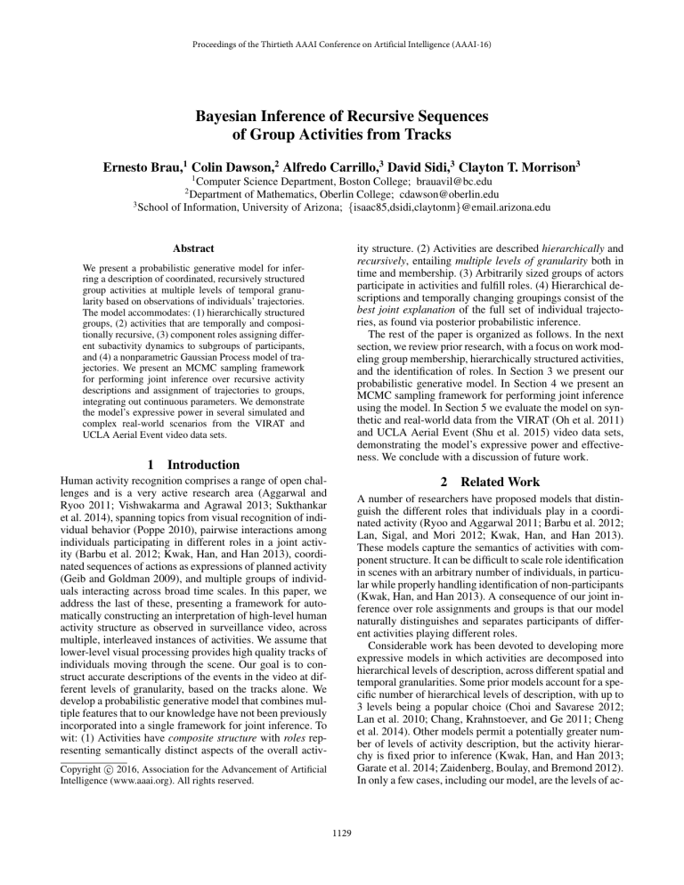
Proceedings of the Thirtieth AAAI Conference on Artificial Intelligence (AAAI-16)
Bayesian Inference of Recursive Sequences
of Group Activities from Tracks
Ernesto Brau,1 Colin Dawson,2 Alfredo Carrillo,3 David Sidi,3 Clayton T. Morrison3
1
Computer Science Department, Boston College; brauavil@bc.edu
Department of Mathematics, Oberlin College; cdawson@oberlin.edu
3
School of Information, University of Arizona; {isaac85,dsidi,claytonm}@email.arizona.edu
2
ity structure. (2) Activities are described hierarchically and
recursively, entailing multiple levels of granularity both in
time and membership. (3) Arbitrarily sized groups of actors
participate in activities and fulfill roles. (4) Hierarchical descriptions and temporally changing groupings consist of the
best joint explanation of the full set of individual trajectories, as found via posterior probabilistic inference.
The rest of the paper is organized as follows. In the next
section, we review prior research, with a focus on work modeling group membership, hierarchically structured activities,
and the identification of roles. In Section 3 we present our
probabilistic generative model. In Section 4 we present an
MCMC sampling framework for performing joint inference
using the model. In Section 5 we evaluate the model on synthetic and real-world data from the VIRAT (Oh et al. 2011)
and UCLA Aerial Event (Shu et al. 2015) video data sets,
demonstrating the model’s expressive power and effectiveness. We conclude with a discussion of future work.
Abstract
We present a probabilistic generative model for inferring a description of coordinated, recursively structured
group activities at multiple levels of temporal granularity based on observations of individuals’ trajectories.
The model accommodates: (1) hierarchically structured
groups, (2) activities that are temporally and compositionally recursive, (3) component roles assigning different subactivity dynamics to subgroups of participants,
and (4) a nonparametric Gaussian Process model of trajectories. We present an MCMC sampling framework
for performing joint inference over recursive activity
descriptions and assignment of trajectories to groups,
integrating out continuous parameters. We demonstrate
the model’s expressive power in several simulated and
complex real-world scenarios from the VIRAT and
UCLA Aerial Event video data sets.
1
Introduction
Human activity recognition comprises a range of open challenges and is a very active research area (Aggarwal and
Ryoo 2011; Vishwakarma and Agrawal 2013; Sukthankar
et al. 2014), spanning topics from visual recognition of individual behavior (Poppe 2010), pairwise interactions among
individuals participating in different roles in a joint activity (Barbu et al. 2012; Kwak, Han, and Han 2013), coordinated sequences of actions as expressions of planned activity
(Geib and Goldman 2009), and multiple groups of individuals interacting across broad time scales. In this paper, we
address the last of these, presenting a framework for automatically constructing an interpretation of high-level human
activity structure as observed in surveillance video, across
multiple, interleaved instances of activities. We assume that
lower-level visual processing provides high quality tracks of
individuals moving through the scene. Our goal is to construct accurate descriptions of the events in the video at different levels of granularity, based on the tracks alone. We
develop a probabilistic generative model that combines multiple features that to our knowledge have not been previously
incorporated into a single framework for joint inference. To
wit: (1) Activities have composite structure with roles representing semantically distinct aspects of the overall activ-
2
Related Work
A number of researchers have proposed models that distinguish the different roles that individuals play in a coordinated activity (Ryoo and Aggarwal 2011; Barbu et al. 2012;
Lan, Sigal, and Mori 2012; Kwak, Han, and Han 2013).
These models capture the semantics of activities with component structure. It can be difficult to scale role identification
in scenes with an arbitrary number of individuals, in particular while properly handling identification of non-participants
(Kwak, Han, and Han 2013). A consequence of our joint inference over role assignments and groups is that our model
naturally distinguishes and separates participants of different activities playing different roles.
Considerable work has been devoted to developing more
expressive models in which activities are decomposed into
hierarchical levels of description, across different spatial and
temporal granularities. Some prior models account for a specific number of hierarchical levels of description, with up to
3 levels being a popular choice (Choi and Savarese 2012;
Lan et al. 2010; Chang, Krahnstoever, and Ge 2011; Cheng
et al. 2014). Other models permit a potentially greater number of levels of activity description, but the activity hierarchy is fixed prior to inference (Kwak, Han, and Han 2013;
Garate et al. 2014; Zaidenberg, Boulay, and Bremond 2012).
In only a few cases, including our model, are the levels of ac-
c 2016, Association for the Advancement of Artificial
Copyright Intelligence (www.aaai.org). All rights reserved.
1129
#
!
"
(b) t = 5
(a) Example activity tree
(c) t = 20
Figure 1: This example depicts five synthetic trajectories and the corresponding activity tree representation. Each node in
the activity tree (a) represents an activity. The central label indicates the activity name, with the time interval for the activity
underneath. Each node is also numbered with a unique ID, which is displayed in the bottom-right corner of each node rectangle.
Shaded nodes indicate physical activities. The outer rectangles represent activity sequences, whose roles and set of participants
are displayed in the top left corner of their rectangles. For example, node 2 is activity C2 with label a2 = MEET, start time
s2 = 1, and end time e2 = 10. Node 2 is part of an activity sequence realizing the role of APPROACHER by individuals
Z2 = {1, 2, 3, 4}. In (b) and (c) we show two frames of the corresponding scene. Each circle represents an individual (1–5),
and the curves are their paths on the ground plane. The dotted rectangles represent activities performed by the individuals inside
them, labeled with their activity name and activity tree node number. For example, we can see in (b), at time t = 5, individuals 1
and 2 are walking together (node 4) to meet (node 2) with individuals 3 and 4, who are standing (node 5). All this happens while
all individuals are participating in another global meeting together (node 1). By frame t = 20, depicted in (c), all participants
are meeting. (Note: to simplify the presentation here, we omit the root FFA activity from the example activity tree in (a).)
tivity description assessed during inference (Lin et al. 2010;
Ryoo and Aggarwal 2011).
A third branch of work has been devoted to modeling activities not just among individuals, but involving groups of
actors. In some models, activities include groups, but interactions are still considered between individuals within
groups (Choi and Savarese 2012; Lan et al. 2010; Zhang
et al. 2013; Odashima et al. 2012; Zhu et al. 2011). Other
models allow for activities to be performed between groups
themselves (Chang, Krahnstoever, and Ge 2011; Chang et al.
2010). Still others, including our model, take group activity
modeling a step further, allowing for arbitrary numbers of
participants in groups, provided they satisfy group membership criteria while performing the activity (Lin et al. 2010;
Kwak, Han, and Han 2013; Shu et al. 2015; Zhang et al.
2012).
Two recent papers, one by Ryoo and Aggarwal (2011) and
one by Shu et al. (2015), come closest to accommodating the
combination of features in our model. Both have developed
methods for simultaneous inference of group structure with
roles in hierarchically structured activities. One key difference between the two is that the former, like our model, can
flexibly accommodate multiple levels of activity description
in the course of inference, while the latter is restricted to two
fixed levels of description during inference (one for group
activities, and the other for their member roles). A crucial
difference with our approach is that we consider the possi-
bility of detecting multiple occurrences of the same type of
activity description in a scene, and these descriptions are integrated into a single probabilistic joint model in order to
influence inference of the overall activity structure. While
activities described in Ryoo and Aggarwal (2011) have hierarchical component structure with roles, their model does
not accommodate more than one top level activity (i.e. assault, meet, robbery, etc.) occurring during the course of the
video, nor changes in group membership by individuals over
such high-level activities.
3
Model
We present a probabilistic generative model describing how
coordinated activities by groups of individuals give rise to
the observed physical trajectories of the actors involved. In
Section 3.1 we introduce some terminology. Then, in Section 3.2 we give precise definitions of the representations
employed by our model for activities, groups, activity sequences, and spatial trajectories. Next, in Section 3.3, we define the factors in the joint probability distribution that comprise the generative model. Finally, in Section 3.4 we define
the specific activities that are used to model the scenes that
we use for evaluation in Section 5.
3.1
Terminology
Activities are optionally composed of other activities. For example, the canonical MEET activity in our model consists of
1130
a RUN activity is expected to yield trajectories with speeds
corresponding to typical human running. We denote the set
of physical activity labels by Aphys . Similarly, intentional
activities include MEET and MOVE - TO. We denote the set
of intentional activity labels by Aint . The complete set of
activities is denoted by A = Aphys ∪ Aint .
multiple participating groups, each of which must MOVE - TO
the location of the meeting, unless they are already there, and
then possibly wait (STAND) until one or more other groups
arrive. Engaging in a MOVE - TO activity requires the group
to carry out a sequence of WALK and RUN activities. The semantics of a WALK or RUN is, in turn, characterized by the
group’s physical trajectory in space.
A scene is described as an activity tree, which has a recursive structure, much as a syntactic tree describes the recursive phrase structure of a natural language sentence, but
with an added temporal component. An example of such a
tree is depicted in Figure 1(a). We refer to the more abstract,
“nonterminal” activities that are defined in terms of other
activities as intentional, and the “leaf” activities that are defined in terms of observable movement as physical.
Participants in an intentional activity are divided into subgroups, each of which plays a particular role with respect to
the parent activity. Carrying out a particular role entails engaging in a sequence of subactivities, each of which may be
physical or intentional. In intentional activities, the group
may be decomposed further into smaller subgroups, each
with their own role in the subactivity, and so on. The sequence of subactivities performed by participants in a role
is constrained (either deterministically or stochastically) according to the dynamics associated with the role. In cases
where a role in a parent activity may be realized as a sequence that includes the same activity type as the parent,
the structure is recursive, and allows for arbitrary nesting of
activities at different time scales. For example, in Figure 1,
a group of individuals participating in a MEET activity performs a sub-MEET of their own.
Physical activities are associated with group trajectories,
which are coupled either via shared membership or when
an intentional activity requires their coordination. An individual, j, has an observed trajectory that is generated as a
sequence of connected sub-trajectories, one for each physical activity in which j participates, and which is constrained
to be near the respective group trajectory. An example of
an observed set of individual trajectories is shown in Figure
1(c).
An important feature of our model is that group trajectories are not explicitly represented during inference. The
assertion that there is some group trajectory induces correlations among the individual trajectories of the members, but
we average over all possible group trajectories (marginalizing them out) when computing the posterior probability of a
description. This allows activity descriptions with different
numbers of groups to be compared based on the posterior
probabilities of their activity trees alone, without needing to
deal with probability densities with different numbers of dimensions.
3.2
Groups The set of participants in activity C is denoted by
ZC ⊂ N. We let JC = |ZC |, the size of the group. This
set is partitioned into subgroups, {Z1 , . . . , ZKC }, where the
number KC of subgroups is bounded only by the number of
individuals, JC , in the group. When specifying the probability model, it is convenient to work instead with the indicator variables, zC = (zC1 , . . . , zCJC ), where zCj indicates
which of the KC subgroups participant j is affiliated with.
Note that zC contains exactly the same information as the
partition. In the following description, we omit the subscript
C for readability.
Activity Sequences Each subgroup within activity C performs a sequence of subactivities. For example, a subgroup
in a MEET might perform a sequence of two subactivities: first, MOVE - TO a designated meeting location, and then
STAND in that location while meeting with other subgroups,
who may have also approached that location. Alternatively,
one of the subgroups could be involved in a side meeting,
with further subgroups that approach and merge with each
other before their union merges with another subgroup of
the top-level MEET. Figure 1 provides such an example.
The sequences of subactivities performed by subgroups
are governed by roles. Each subgroup k is assigned a role
from a set Ra defined by the parent activity a. Roles govern the dynamics of the sequence of subactivities that each
group carries out, via a set of parameters associated with
that role. The parameters for role r specify what the allowable activities are in the activity sequence of a group carrying out that role, as well as hard or soft constraints involving what order the activities occur in. The subgroup of the
example MEET activity above would be assigned the role of
APPROACHER, which prescribes a MOVE - TO followed by
a STAND. In this case the constraint on the order of subactivities is deterministic, with the only degrees of freedom being
the times at which transitions take place. These constraints
can be represented by a Markov chain with a degenerate initial distribution and a transition matrix with only one nonzero off-diagonal entry per column. More general initial and
transition distributions will give rise to softer constraints on
activity sequences.
Trajectories Ultimately, each physical activity, realized
over the interval [s, e], is associated with a group trajectory,
denoted by x, which is a 2 by e − s + 1 array specifying a 2-dimensional position on the ground plane for each
time index between s and e inclusive. The group trajectory
represents the central tendency of the members’ individual
trajectory segments during the interval [s, e]. Since individual j’s path depends on the sequence of activities it participates in, each individual trajectory yj consists of seg(I )
(0)
ments, yj , . . . , yj j , consecutive pairs of which must be
Representation
Activities Formally, an activity is a tuple C = (a, s, e),
where a is an activity label (e.g., WALK), and s, e ∈ R+
are the start and end time of the activity, respectively. The
simplest activities are physical activities, e.g., walking, running and standing, which directly constrain the motion of a
group of individuals over an interval of time. For example,
1131
(1)
(I )
(i)
connected at transition points, y∗j , . . . , y∗jj , where y∗j denotes the start of segment i and the end of segment i − 1.
3.3
Cm
Generative Model
Cm1 , Zm1
We now describe the generative process for activities. The
high-level process has three steps: (1) recursive expansion of
intentional activities, (2) generation of group trajectories for
the set of physical activities, and (3) generation of individual
trajectories conditioned on the group assignments and group
trajectories.
(0)
Cm1
CmKm , ZmKm
(I
Cm1m1
)
(0)
CmKm
(I
mKm
CmK
m
)
Figure 2: Graphical model for an intentional activity. The set
Zm of participants of activity Cm is partitioned into groups
Zm1 , . . . ZmKm via the indicator vector zm . Each group
is assigned a role, rmk , and performs an activity sequence
(0)
(I
)
Cmk = (Cmk , . . . , Cmkmk ), k = 1, . . . , Km .
Overview In the first step of activity generation, each intentional activity gives rise to one or more child activity sequences: one for each subgroup of participants involved in
the parent activity. Each child sequence is assigned a role,
based on the parent activity type. Subgroups and role assignments occur jointly. The choice of role governs the sequence
of activities that the subgroup engages in, by specifying a
Markov transition function. Each segment of an activity sequence may be a physical activity or another intentional activity. Each intentional activity in the sequence is recursively
expanded until only physical activities are generated.
As a working example for this stage of the process, we
consider the MEET activity at node 1, at the root of the tree in
Figure 1(a). Node 1 has two child sequences corresponding
to the two subgroups involved in the meeting, both carrying
out the APPROACHER role. One of those child sequences
consists of just a single MOVE - TO activity, while the other
consists of two activities: a MEET, followed by a MOVE - TO.
In general, a special top-level root activity, a “free-for-all”
(FFA), comprises all actors and has a duration over the entire video. All other activities are children of the root FFA.
(To simplify the example tree in Figure 1(a), we removed
the parent FFA.) The details of this tree expansion are given
in “Generating the Activity Tree”, below.
We make a conditional independence assumption by supposing that the contents of a parent activity fully specify the
distribution of possible child sequences, and that child sequences are conditionally independent of each other given
their parent. Since child sequences can contain other intentional activities, activity generation is a recursive process,
which bottoms out when no intentional activities are generated.
In the second step of the generative process, group trajectories are generated for each physical activity. This process
must satisfy two constraints: (a) physical activity trajectories
that share members and that border in time must be spatially
connected; and (b) groups that need to physically interact
as co-participants in an intentional activity, such as a MEET,
must have trajectories that intersect at the appropriate points
in time. Due to these constraints it is not feasible to generate group trajectories conditionally independently given the
activity tree. Instead they are generated jointly according to
a global Gaussian Process with a covariance kernel that depends on the activity tree in such a way as to enforce the key
constraints. The details of this process are given in “Generating Group Trajectories”, below.
For the example tree in Figure 1(a), four group trajectory segments are needed, one for each physical activity leaf
node. Since WALK activity 9 is part of a meeting in which
its participants must meet with the participants in WALK activity 7, the group trajectories for 7 and 9 must end in the
same location. Similarly, WALK 4 must end where STAND 5
is located.
In the final step of the generative process, the individual
trajectories are realized, conditioned on the set of group trajectories. Here, conditional independence is possible, with
each individual’s trajectory depending only on the sequence
of group trajectories for physical activities in which that individual is a participant. This process is detailed in Section
“Generating Individual Trajectories”.
Generating the Activity Tree Let Cm = (am , sm , em )
be a parent intentional activity, where m indexes the set of
activities. Its participant set Zm (by relabeling, we assume
that Zm = {1, . . . , Jm }) is divided into subgroups, where
the jth participant of Cm is assigned to group zmj , and the
distinct realized groups are numbered 1 through Km . We let
zm = (zm1 , . . . , zmJm ), which defines a partition of Zm
into Km subgroups, {Zm1 , . . . , ZmKm }, with Zmk = {j ∈
Zm | zmj = k}. Subgroup k is assigned role rmk ∈ R, and
we define rm = (rm1 , . . . , rmKm ).
The kth subgroup, which has participants Zmk and role
rmk , produces an activity sequence according to the stochastic process associated with rmk , which has parameters πrmk ,
a Markov transition function, and Trmk , an initial activity distribution. Denote the resulting sequence by Cmk =
(0)
(I
)
(Cmk , . . . , Cmkmk ), where Imk is the number of jumps gen(i)
erated by the process, and the Cmk are activity tuples,
(i)
(i)
(i)
(i)
(i)
(i−1)
Cmk = (amk , smk , emk ), where smk = emk . Figure 2
illustrates the graphical model of this production.
To summarize, the grouping, role assignment, and child
activity sequences within activity Cm are generated according to p(zm , rm , Cm | Cm , Zm ), which factors as
p(zm | am , Zm )p(rm | am )
K
m
p(Cmk | sm , em ),
(1)
k=1
where we define Cm = (Cm1 , . . . , CmKm ). We assume
that roles are assigned independently, so that p(rm | am ) =
K m
k=1 p(rmk | am ). Additionally, we model the partition of
Zm into subgroups using a Chinese Restaurant Process
(CRP), whose concentration parameter αam depends on
1132
the activity label. That is, we let p(zm | am , Zm ) be the
CRP mass function with parameter αam . Each segment
(i)
Cmk of Cmk that is an intentional activity is expanded
and its members are subdivided recursively according to
(i)
(1), replacing Cm with Cmk and Zm with Zmk . Once all
expansions contain exclusively physical activities, the recursion has bottomed out. The resulting tree consists of
all intentional activities C1 , . . . , CM , all physical activities, CM +1 , . . . , CM +N , and, for each intentional activity
m = 1, . . . , M , its membership partition zm , role assignments rm , and subgroup activity sequences Cm . We denote
this complete tree by Λ, whose prior distribution is
p(Λ) =
M
p(zm , rm , Cm | Cm , Zm ).
of the time elapsed during the intervening physical activity
and the σ associated with the activity label (e.g., “slowermoving” activities having lower weights, corresponding to
a stronger dependence between the positions of their endpoints). Figure 3 shows an example G.
(2)
m=1
Generating Group Trajectories The leaves of the activity tree are all physical activities, each of which is associated
with a group trajectory. In general, the endpoints of different
group trajectories are not independent (given Λ), since they
may be constrained to start or end at the same location. Consequently, we define a joint distribution on all of the group
trajectory endpoints, and, conditioned on their endpoints, we
treat their interiors as independent.
We model the interiors as realizations of Gaussian processes (Rasmussen and Williams 2006) with the squaredexponential kernel function. This results in trajectories that
are generally smooth, but flexible enough to allow for different kinds of motion. We use different scale parameters σam
depending on the activity am , which determines the rate of
change of the trajectory.
We specify dependencies among the set of trajectory endpoints by first defining an undirected weighted graph G over
the endpoints. We use this graph to construct a constraint
matrix over transition points by interpreting the sum of the
weights on the shortest path between two nodes as distances.
We then apply a positive semidefinite isotropic covariance
kernel point-wise to the distance matrix to transform the distances into covariances.
Let xm ∈ R2(em −sm +1) represent the sequence of
ground-plane positions that make up the group trajectory for
(s)
activity m. Abusing notation slightly, we will write x∗m and
(e)
x∗m for both the endpoints of a group trajectory and the corresponding node in G. We introduce three kinds of edges
on G: temporal, transitional, and compositional. Two nodes
are connected by a temporal edge when they belong to the
(s)
same physical activity. The start of an activity, x∗m , is con(e)
nected to the end of another activity, x∗m , by a transitional
edge when they correspond to the same moment in time and
the corresponding activities share at least one participant. Finally, two endpoints are connected by a compositional edge
if they correspond to the same moment in time and have a
common ancestor that specifies they must coincide, e.g., in
a MEET activity, all participants must end in the same location. All transitional and compositional edges have weight
(or “distance”) zero, corresponding to the constraint that the
connected edges must correspond to the same trajectory position. The weight assigned to temporal edges is a function
Figure 3: Constraint graph for the example activity tree in
Figure 1. The nodes in the graph represent endpoints for
group trajectories, labeled according to the numbering in
(s)
the tree; e.g., x∗9 is the starting endpoint for node 9. Solid
lines represent temporal edges, dashed lines are transitional
edges, and dotted lines are compositional edges (see Section
3.3, “Generating Group Trajectories”). For clarity, temporal
edges are labeled with their corresponding physical activ(s)
ity name. According to this graph, the distance between x∗5
(s)
and x∗9 is w5 +w7 +w9 , meaning that activities 5 and 9 must
start in locations separated by a STAND and two WALKs.
Having defined G we can compute a distance matrix D for
the set of physical activity endpoints, where the entry dii is
the sum of the weights along the shortest path in G from node
i to node i . If no path exists between two nodes, the distance
is set to ∞. We then transform D into a covariance matrix
Φ by applying the covariance function φii = κ(dii ) =
2
λe−dii . The locations of the set of group trajectory end(s)
(e)
(s)
(e)
points X∗ = (x∗M +1 , x∗M +1 , . . . , x∗M +N , x∗M +N ) is distributed as X∗ | Λ ∼ N (0, Φ). Conditioned on the endpoints, the interiors are mutually independent, so that
p(X−∗ | X∗ ) =
M
+N
(s)
(e)
p(x−∗m | x∗m , x∗m ),
(3)
m=M +1
where x−∗m is the vector of interior points of trajectory
xm and X−∗ = (x−∗M +1 , . . . , x−∗M +N ). Each x−∗m
is generated according to the Gaussian process for activ(s)
(e)
ity m; i.e., x−∗m | x∗m , x∗m is normally distributed. Finally, the distribution over the physical trajectories X =
(xM +1 , . . . , xM +N ) factorizes as
p(X | Λ) = p(X−∗ | X∗ )p(X∗ | Λ).
(4)
Using the fact that factors in (4) are normally distributed, we
can easily see that X also has a normal distribution.
Generating Individual Trajectories As described above,
individual j participates in physical activity sequence C(j) ,
which has the sequence of group trajectories Xj =
(I )
(1)
(xj , . . . , xj j ). The individual trajectory yj consists of
1133
Cm
Zm1
Zn1
(0)
(1)
Cm1
(0)
Zn2
(0)
Cm1
(0)
Cn1
(1)
xm1
a MEETs (recursively) and MOVE - TOs, and a WAITER
only performs STANDs. M OVE - TO only produces one role,
MOVER, which switches uniformly at random between the
three physical activities. Finally, the physical activities have
scale parameters such that σSTAND < σWALK < σRUN .
Cn
Cn2
(0)
xm1
4
(0)
xn1
Inference
Given a set of J individual trajectories Y = (y1 , . . . , yJ ),
such as those depicted in Figure 1(c), we wish to find an activity tree Λ, such as that depicted in Figure 1(a), that best
describes them. Specifically, we wish to maximize the posterior probability of an activity tree given the observed data
xn2
p(Λ | Y) ∝ p(Λ)p(Y | Λ),
y1
where the prior is given by (2), and the likelihood is
J
p(Y | Λ) = p(X | Λ)
p(yj | Xj , Cj ) dX.
y2
Figure 4: Graphical model for the generation of trajectories.
This example shows a sequence of activities with two activities Cm and Cn . Cm has a single child with individuals Zm1 performing a sequence of two physical activities
(0)
(1)
Cm1 and Cm1 , while Cn is divided into two groups, each of
which performs a single activity, culminating in physical ac(0)
(0)
tivities Cn1 and Cn2 . Each corresponding group trajectory
(0)
(1)
(0)
(0)
xm1 , xm1 , xn1 , and xn2 potentially depends on all physical
activities, as well as being fully connected with each other
(represented in the graph by thick red edges). Finally, individual trajectories y1 and y2 only depend on group trajectories whose physical activities contained their individuals.
(Ij )
(1)
segments, yj , . . . , yj
(i)
The integrands are given by (4) and (5). In general, the integral in (7) cannot be computed analytically. However, since
every factor in (7) is a normal pdf, p(Y | Λ) is also normal,
which makes the evaluation of (6) straightforward.
We cannot find Λ∗ = arg maxΛ p(Λ | Y) analytically. Instead, we draw S samples from the posterior (6) using the
Metropolis-Hastings (MH) algorithm, and keep the sample
with the highest posterior probability. At the ith iteration,
we draw Λ from a proposal distribution q(· | Λ(i−1) ), where
Λ(i−1) is the current sample, and accept the sample with the
standard MH acceptance probability (Neal 1993).
The ability of MH to efficiently explore the space depends largely on the choice of the proposal distribution
q. Although there has been work on MCMC sampling
on tree models (Chipman, George, and McCulloch 2002;
Pratola 2013) there is no general approach which can be
applied to any model. Consequently, we employ a proposal
distribution which is specific to our model.
(i)
poral interval as xj . Given these group trajectories, the individual trajectory segments are mutually independent, so
that
p(yj | Xj , C(j) ) =
(i)
(i)
(i)
p(yj | xj , a(j) ),
4.1
(5)
is the label of the ith activity in sequence C(j) .
where
We also use a Gaussian process for individual trajectories,
(i)
but fix the mean to the (given) group trajectory, i.e. yj ∼
(i)
(i)
(i)
where the ijth entry in Kj
(i)
(i)
∼ N (xj , Kj ),
is the covariance function κ
(i)
evaluated at the ith and jth frames of yj , using the scale
(i)
corresponding to the activity label associated to xj . See
Figure 4 for an example graphical model of this distribution.
3.4
Proposal distribution
Our proposal mechanism is composed of sampling moves
which perform edits to the current hypothesized activity tree
to produce a new tree sample. When drawing a sample from
q, we choose a move uniformly at random to apply. When
applying a move, we must make sure that the resulting tree is
valid (e.g., start and end times must be consistent; or activity
sequences must be possible given the role), which requires
book-keeping that is beyond the scope of this document.
We have also developed a set of bottom-up activity detectors to help explore the space efficiently. These detectors provide rough estimates of groupings of individuals at
each frame, and activities being performed by each group
(see Section 4.1, “Detectors”). We use these detectors in two
ways. First, we initialize the sampler to a state obtained by
transforming the output of the detectors to an activity tree
Λ(0) . Additionally, we bias our proposal distribution toward
groups and activities found by the detectors. For example,
when proposing a merge move, we might choose participants which are predicted to be in a group by some activity
detector.
i=1
(i)
a(j)
GP(xj , κ), which implies that yj
(7)
j=1
, where yj spans the same tem-
Ij
(6)
Specific Activities
In this work, we limit ourselves to six specific activities,
three intentional (FREE - FOR - ALL, MEET, and MOVE - TO)
and three physical (STAND, WALK, and RUN). FFA has
a single role which allows all activities to take place. A
MEET activity assigns non-zero probability to two roles, APPROACHER and WAITER; an APPROACHER performs
1134
Cm
Cm
Cm1
C
CmKm
Cm1
Cm
CmKm
Zmk
(0)
Cmk
(a) Birth/death
Cm
Cm
Zmk
Cmk , Zmk
Zmk
(0)
Cmk
Cm
(0)
(0)
Cmk
Cmk
C
(I )
Cmkk
(0)
Cmk
(b) Merge/split
mk
,Z
mk
(I
)
Cmkk
(Cmk , C
mk
), Zmk ∪ Z
mk
(0)
Cmk
(I )
Cmkk
(0)
Cmk
(I
Cmkk
)
(c) Sequence/unsequence
Figure 5: An illustration of our sampling moves. (a) The birth move (left to right) inserts an intentional activity C between
sequences Cm1 , . . . , CmKm and their parent Cm . In the death move, the opposite operation is performed. (b) In the merge
(0)
(0)
move (left to right), children Cmk and Cmk of intentional activity Cm (and members of single-activity sequences), with
(0)
(0)
(0)
(0)
amk = amk , are replaced by a single activity node Cmk , with activity amk , and participant set Zmk ∪ Zmk . In the reverse
(0)
(0)
move, Cmk is split into two nodes, both with activity label amk , with Zm randomly partitioned. (c) In this example, a sequence
move (left to right) takes two child sequences of intentional activity node Cm , Cmk and Cmk , and forms a single sequence
(Cmk , Cmk ) with participant set Zmk ∪ Zmk . In the reverse move, we randomly choose a split point in the activity sequence
on the right, and create two separate sequences under the same parent Cm .
Sampling moves During inference, we employ the following moves (see Figure 5 for an illustration). (a)
Birth/death: a birth move inserts an intentional activity
node between an intentional activity and some of its children. We randomly choose a set of sibling activity sequences
Cm1 , . . . , CmKm whose parent is intentional activity Cm ,
and insert a new intentional activity node C (whose label
is also chosen at random), such that C becomes the parent
of Cm1 , . . . , CmKm and a child of Cm . In a death move,
we randomly choose a intentional node C , remove it from
the tree, and connect its children nodes to its parent. (b)
Merge/split: In a merge move, we take two sibling activity
nodes with the same label and combine them into a single activity. If C and C are two activities with label a and groups
Z and Z , we create a new node C with label a and participants Z ∪ Z . The split move performs the opposite operation, taking a-labeled node C and splitting it into two nodes
C and C , both with activity a, assigning participants in
Z to either Z or Z uniformly. (c) Sequence/unsequence:
Let C1 and C2 be two temporally non-overlapping sibling
activity sequences. A sequence move concatenates C1 and
C2 into a new sequence C. An unsequence move randomly
selecting a split point at which to separate a sequence. (d)
Relabel move: The relabel move randomly changes C’s label. Note that the label must be valid, e.g., we cannot assign
a physical activity label to an intentional activity node.
uals in that new set are still involved. Given the groups as
computed above, we want to identify the physical activities
of their individuals (e.g., WALK , RUN). For this we use a
hidden Markov model, where the observation function is a
naive Bayes model with each individual’s speed modeled by
a Gamma distribution, and a transition function that prefers
staying within the current activity.
5
Experiments and Results
We evaluate the model in two ways. First, we demonstrate
the model’s expressive power in inferring two different types
of complexly structured scenarios from synthetic data. In the
first, groups of individuals engage in activities and disband,
forming different groups over time. The second demonstrates a recursively structured activity, in which one meeting is a component of a higher-level meeting. We then evaluate the model on real data; specifically on two publicly available group activity datasets, VIRAT (Oh et al. 2011) and the
UCLA aerial event dataset (Shu et al. 2015).
5.1
Evaluation
Performance is measured in terms of how well activities are
labeled in the scene, and how well individuals are grouped,
irrespective of activity label. In the following, Λgt and Λ are
the ground truth and inferred activity trees, respectively.
Activity Labeling For each activity a and video frame f ,
we compare between Λgt and Λ the set of individuals performing a at f . We first define performance counts in terms
of an individual at a frame, then compute overall counts and
associated performance measures.
For an individual j at frame i, let λji be the set of individuals which have the same label as j in Λ. Define λji
similarly for Λgt . The set of false positives for j is λji \ λji ,
the set of false negatives is λji \ λji, the true positives are
λji ∩ λji , and the true negatives are (Z \ λji ) ∩ (Z \ λji ),
where Z is the set of all individuals.
Detectors The bottom-up detectors provide an estimate of
how individuals in the video are grouped across time, as well
as the physical activity they are performing.
At each frame, we cluster individuals into groups using their trajectories on the ground plane. We apply the
density-based spatial clustering of applications with noise
(DBSCAN) (Ester et al. 1996) algorithm independently on
each frame, where our feature is composed of the position
and velocity of an individual at that frame, both of which
are obtained from the smoothed trajectories (which are assumed to be given). Importantly, we keep track of individual identities over time by recording the actors involved in
each group in the previous frame and assigning the cluster
found in the following frame where the majority of individ-
Grouping We follow a similar approach when evaluating
grouping performance. For person j, we compare the groups
to which j belongs in Λgt and Λ at each frame t. Since the
1135
(a) VIRAT frames
(b) Inferred activity tree
WALK
0.84
0.94
0.88
MOVE-TO
0.63
0.71
0.67
MEET
0.71
0.75
0.73
FFA
1.00
1.00
1.00
SYNTH2
Precision
Recall
F1
STAND
0.87
0.50
0.63
WALK
1.00
0.71
0.83
MOVE-TO
0.94
0.73
0.82
MEET
1.00
0.56
0.72
FFA
×
×
×
VIRAT
Precision
Recall
F1
STAND
0.85
0.51
0.64
WALK
0.81
0.88
0.85
MOVE-TO
0.73
0.89
0.81
MEET
0.90
0.80
0.85
FFA
1.0
1.0
1.0
UAED
Precision
Recall
F1
STAND
0.96
0.82
0.86
WALK
0.89
0.99
0.94
MOVE-TO
0.71
0.67
0.62
MEET
0.75
0.64
0.62
FFA
0.97
0.73
0.77
Table 1: Activity labeling results for synthetic videos
SYNTH1 and SYNTH2, and the VIRAT and UCLA aerial
event datasets. Each table shows precision, recall, and F1 for
each activity. See Section 5.1 for details.
Figure 6: Qualitative results the VIRAT dataset. (a) shows
two frames of the VIRAT2 video. Red boxes represent
tracked individuals, gray rectangles indicate groups of individuals, and white boxes contain information such as track
id, etc. In (b) we show the inferred activity tree, illustrated
in a similar way as in Figure 1(a).
Precision
Recall
F1
two trees could have different depths and topologies, it is
not necessarily clear which groups should be compared with
which; however, every individual is part of exactly one physical activity group at each frame, as well as one highest level
node. Consequently, we only compare groups at these two
levels of the tree, without penalty for difference in activities
within a level. Thus once we determine the group associated with person j at frame t at the physical (resp. highest)
activity level of each tree, we compute the score as before.
5.2
STAND
0.59
1.00
0.74
SYNTH1
Precision
Recall
F1
SYNTH1
PHYS INT
0.86
1.0
1.00
1.0
0.92
1.0
SYNTH2
PHYS INT
1.00
1.0
0.69
1.0
0.82
1.0
VIRAT
PHYS INT
0.98
1.0
0.85
1.0
0.91
1.0
UAED
PHYS INT
0.95
0.93
0.99
0.89
0.97
0.89
Table 2: Grouping precision, recall, and F1 scores for the
synthetic videos and the two datasets VIRAT and UCLA
aerial event dataset (UAED). See Section 5.1 for details.
frames of the video, along with the inferred activity tree.
Our model correctly recognizes the two meetings, as well
as all of the groups at the highest level of description. The
activity labeling results (Table 1) show perfect FFA performance, and the grouping results (Table 2) show a perfect
highest-level intentional activity score. As before, there is
divergence from ground truth at the physical activity level,
but this does not affect the grouping score.
Results
The performance of our algorithm is summarized in Tables
1 and 2. Table 1 shows the activity labeling precision and
recall on the two synthetic scenes (SYNTH1 and SYNTH2),
a video sequence obtained from the VIRAT dataset, and
four different video sequences from the UCLA aerial event
dataset (UAED). In Table 2 we see the performance as measured by our grouping evaluation metric described above.
UCLA aerial event dataset We extracted four video sequences from the UCLA aerial event dataset (UAED). More
specifically, we searched for subsequences of videos which
featured properties like activity nesting, groups interchanging members, etc. The result is four video sequences of
roughly 2000 frames each. As we can see in Table 1, which
shows the overall precision and recall scores, for all four
videos, our algorithm performs reasonably well across all
activities. Note the relatively low recall score of the MEET
activity, which is due in large part to one very long missed
MEET in the third video sequence. Similarly, Table 2 shows
that our algorithm performs well at finding groups of individuals at both the physical and intentional activity levels.
Synthetic data The synthetic dataset comprises two
videos, where a video is a set of trajectories on the ground
plane. In the first, SYNTH1, five actors participate in a series of meetings, where participants repeatedly change group
memberships across 20 frames. The second (SYNTH2) features five actors meeting, with four of them participating in
a side meeting before joining the global meeting. As Table
1 shows, our model performs very well on high-level activities, such as MEET, even when presented with nested structure.
6
VIRAT We also evaluate on real data, specifically frames
2520 to 3960 of video 2 of the VIRAT dataset. This video
features seven people participating in two meetings, where
groups exchange members several times. Fig. 6 shows two
Discussion
We have presented a probabilistic generative model of complex multi-agent activities over arbitrary time scales. The activities specify component roles between groups of actors
1136
and accommodate unboundedly deep recursive, hierarchical
structure. The model accommodates arbitrary groups participating in activity roles, describing both between-group
and between-individual interactions. Physical and intentional (higher-level description) activities explain hierarchical correlations among individual trajectories. To our knowledge, no existing model of track-based activity recognition
provides this expressiveness in a joint model.
The modeling framework is naturally extensible. We are
currently undertaking several extensions, including (1) developing additional activities, including following, exchanging items, and interacting with vehicles and building entrances, (2) adding prior knowledge about the spatial layout of the scene that naturally constrains what activities are
possible, such as roads, sidewalks, impassible buildings, and
other spatial features that influence behavior in order to improve both accuracy and speed by reducing the search space,
(3) using our model as a prior for a 3D Bayesian tracker
(Brau et al. 2013), and (4) connecting natural language to activity descriptions as our model accommodates activity descriptions across multiple events, tracking individual participation throughout, providing opportunities for building natural language narratives about activities at different levels of
granularity.
Ester, M.; peter Kriegel, H.; S, J.; and Xu, X. 1996. A densitybased algorithm for discovering clusters in large spatial databases
with noise. 226–231. AAAI Press.
Garate, C.; Zaidenberg, S.; Badie, J.; and Bremond, F. 2014. Group
tracking and behavior recognition in long video surveillance sequences. In VISIGRAPP 2014.
Geib, C. W., and Goldman, R. P. 2009. A probabilistic plan recognition algorithm based on plan tree grammars. Artificial Intelligence 173:1101–1132.
Kwak, S.; Han, B.; and Han, J. H. 2013. Multi-agent event detection: localization and role assignment. In CVPR.
Lan, T.; Wang, Y.; Yang, W.; and Mori, G. 2010. Beyond actions:
Discriminative models for contextual group activities. In Advances
in neural information processing systems, 1216–1224.
Lan, T.; Sigal, L.; and Mori, G. 2012. Social roles in hierarchical
models for human activity recognition. In CVPR.
Lin, W.; Sun, M.-T.; Poovendran, R.; and Zhang, Z. 2010. Group
event detection with a varying number of group members for video
surveillance. Circuits and Systems for Video Technology, IEEE
Transactions on 20(8):1057–1067.
Neal, R. M. 1993. Probabilistic inference using markov chain
monte carlo methods. Technical report.
Odashima, S.; Shimosaka, M.; Kaneko, T.; Fukui, R.; and Sato, T.
2012. Collective activity localization with contextual spatial pyramid. In Computer Vision–ECCV 2012. Workshops and Demonstrations, 243–252. Springer.
Oh, S.; Hoogs, A.; Perera, A.; Cuntoor, N.; Chen, C.-C.; Lee, J. T.;
Mukherjee, S.; Aggarwal, J.; Lee, H.; Davis, L.; et al. 2011. A
large-scale benchmark dataset for event recognition in surveillance
video. In CVPR 2011, 3153–3160. IEEE.
Poppe, R. 2010. A survey on vision-based human action recongition. Journal of Image and Vision Computing 28(6):976–90.
Pratola, M. T. 2013. Efficient metropolis-hastings proposal mechanisms for bayesian regression tree models.
Rasmussen, C. E., and Williams, C. K. I. 2006. Gaussian Processes
for Machine Learning. The MIT Press.
Ryoo, M. S., and Aggarwal, J. K. 2011. Stochastic representation and recognition of high-level group activities. International
Journal of Computer Vision 93(2):183–200.
Shu, T.; Xie, D.; Rothrock, B.; Todorovic, S.; and Zhu, S.-C. 2015.
Joint inference of groups, events and human roles in aerial videos.
In CVPR.
Sukthankar, G.; Goldman, R. P.; Geib, C. W.; Pynadath, D. V.; and
Bui, H. H., eds. 2014. Plan, Activity, and Intent Recognition: Theory and Practice. Morgan Kaufmann.
Vishwakarma, S., and Agrawal, A. 2013. A survey on activity
recognition and behavior understanding in video surveillance. The
Visual Computer 29(10):983–1009.
Zaidenberg, S.; Boulay, B.; and Bremond, F. 2012. A generic
framework for video understanding applied to group behavior
recognition. In AVSS, 136–142. IEEE.
Zhang, C.; Yang, X.; Zhu, J.; and Lin, W. 2012. Parsing collective behaviors by hierarchical model with varying structure. In
ACMMM 2012, 1085–1088. ACM.
Zhang, Y.; Qin, L.; Yao, H.; Xu, P.; and Huang, Q. 2013. Beyond particle flow: Bag of trajectory graphs for dense crowd event
recognition. In ICIP, 3572–3576.
Zhu, G.; Yan, S.; Han, T. X.; and Xu, C. 2011. Generative group
activity analysis with quaternion descriptor. In Advances in Multimedia Modeling. Springer. 1–11.
Acknowledgements
This research was supported by grants under the DARPA
Mind’s Eye program W911NF-10-C-0081 (subcontract to
iRobot, 92003) and the DARPA SSIM program W911NF10-2-0064. We give special thanks to Paul R. Cohen and
Christopher Geyer for helpful discussions and advice.
References
Aggarwal, J. K., and Ryoo, M. S. 2011. Human activity analysis:
A review. ACM Computing Surveys (CSUR) 43(3).
Barbu, A.; Bridge, A.; Burchill, Z.; Coroian, D.; Dickinson, S.;
Fidler, S.; Michaux, A.; Mussman, S.; Siddharth, N.; Salvi, D.;
Schmidt, L.; Shangguan, J.; Siskind, J. M.; Waggoner, J.; Wang,
S.; Wei, J.; Yin, Y.; and Zhang, Z. 2012. Video in sentences out. In
UAI 2012.
Brau, E.; Guan, J.; Simek, K.; del Pero, L.; Dawson, C. R.; and
Barnard, K. 2013. Bayesian 3d tracking from monocular video. In
ICCV 2013.
Chang, M.-C.; Krahnstoever, N.; Lim, S.-N.; and Yu, T. 2010.
Group level activity recognition in crowded environments across
multiple cameras. In AVSS, 56–63.
Chang, M.-C.; Krahnstoever, N.; and Ge, W. 2011. Probabilistic group-level motion analysis and scenario recognition. In ICCV
2011, 747–754. IEEE.
Cheng, Z.; Qin, L.; Huang, Q.; Yan, S.; and Tian, Q. 2014. Recognizing human group action by layered model with multiple cues.
Neurocomputing 136:124–135.
Chipman, H.; George, E.; and McCulloch, R. 2002. Bayesian treed
models. Machine Learning 48(1-3):299–320.
Choi, W., and Savarese, S. 2012. A unified framework for multitarget tracking and collective activity recognition. In ECCV 2012,
215–230.
1137