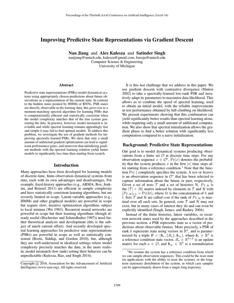
Proceedings of the Thirtieth AAAI Conference on Artificial Intelligence (AAAI-16)
Improving Predictive State Representations via Gradient Descent
Nan Jiang and Alex Kulesza and Satinder Singh
nanjiang@umich.edu, kulesza@gmail.com, baveja@umich.edu
Computer Science & Engineering
University of Michigan
It is this last challenge that we address in this paper: We
use gradient descent with contrastive divergence (Hinton
2002) to take a spectrally-learned low-rank PSR and iteratively adapt its parameters to maximize data likelihood. This
allows us to combine the speed of spectral learning, used
to obtain an initial model, with the reliable improvements
in test performance obtained by hill-climbing on likelihood.
We present experiments showing that this combination can
yield significantly better results than spectral learning alone,
while requiring only a small amount of additional computation. We also show that spectral initialization allows the gradient phase to find a better solution with significantly less
computation compared to a naive initialization.
Abstract
Predictive state representations (PSRs) model dynamical systems using appropriately chosen predictions about future observations as a representation of the current state. In contrast
to the hidden states posited by HMMs or RNNs, PSR states
are directly observable in the training data; this gives rise to a
moment-matching spectral algorithm for learning PSRs that
is computationally efficient and statistically consistent when
the model complexity matches that of the true system generating the data. In practice, however, model mismatch is inevitable and while spectral learning remains appealingly fast
and simple it may fail to find optimal models. To address this
problem, we investigate the use of gradient methods for improving spectrally-learned PSRs. We show that only a small
amount of additional gradient optimization can lead to significant performance gains, and moreover that initializing gradient methods with the spectral learning solution yields better
models in significantly less time than starting from scratch.
Background: Predictive State Representations
Our goal is to model dynamical systems producing observations from a finite set O at discrete time steps. For any
observation sequence x ∈ O∗ , Pr(x) denotes the probability that the system produces x in the first |x| time steps after starting from a reference condition.1 Note that the function Pr(·) completely specifies the system. A test or history
is an observation sequence in O∗ that has been selected to
capture information about the future or past, respectively.
Given a set of tests T and a set of histories H, PT ,H is
the |T | × |H| matrix indexed by elements in T and H with
[PT ,H ]t,h = Pr(ht), where ht is the concatenation of h and
t. Sets T and H are called core if the rank of PT ,H is maximal over all such sets. In general, core T and H may not
exist, but in many cases of interest they do and can even be
explicitly identified (Singh, James, and Rudary 2004).
Instead of the finite histories, latent variables, or recurrent network states used by the approaches described in the
previous section, a PSR represents state as a vector of predictions about observable futures. More precisely, a PSR of
rank k represents state using vectors in Rk , and is parameterized by a triple B = (b∗ , {Bo }, b∞ ), where b∗ ∈ Rk is
a reference condition state vector, Bo ∈ Rk×k is an update
matrix for each o ∈ O, and b∞ ∈ Rk is a normalization
Introduction
Many approaches have been developed for learning models
of discrete-time, finite-observation dynamical systems from
data, each with its own advantages and disadvantages. For
example, fixed-history approaches (e.g., ARMA; Box, Jenkins, and Reinsel 2011) are efficient in sample complexity
and have statistically consistent learning algorithms, but are
severely limited in scope. Latent-variable approaches (e.g.,
HMMs and other graphical models) are powerful in scope
but require slow, iterative optimization algorithms subject
to local minima (Wu 1983). Recurrent neural networks are
powerful in scope but their learning algorithms (though already useful (Hochreiter and Schmidhuber 1997)) need further theoretical analysis and development (this is the subject of much current effort). And recently developed spectral learning approaches for predictive state representations
(PSRs) are powerful in scope as well as statistically consistent (Boots, Siddiqi, and Gordon 2010), but, although
they are well-understood in idealized settings where model
complexity precisely matches the data, in the more realistic model mismatch (low rank) setting their behavior can be
unpredictable (Kulesza, Rao, and Singh 2014).
1
We assume the system has a reference condition from which
we can sample observation sequences. This could be the reset state
(in applications with the ability to reset the system), or the longterm stationary distribution of the system, in which case samples
can be approximately drawn from a single long trajectory.
c 2016, Association for the Advancement of Artificial
Copyright Intelligence (www.aaai.org). All rights reserved.
1709
vector. Let b(h) denote the PSR state after observing history
h from the reference condition (so b() = b∗ , where is the
empty string); the update rule after observing o is given by
b(ho) =
Bo b(h)
b∞ Bo b(h)
.
the learned model approaches the truth may nevertheless be
quite slow. The bound of Hsu, Kakade, and Zhang (2012),
for instance, depends on the smallest nonzero singular value
4
. Thus, for finite training sets, spectrally
of PT ,H as 1/σmin
learned models can be far from optimal. (Intuitively, since
the algorithm depends only on summary statistics of the
data, it cannot be expected to match the statistical efficiency
of optimization-style learning.)
For all of these reasons, our goal is to find effective ways
of improving the real-world performance of spectral learning for PSRs. The solution we offer in this paper is to use
spectral learning to initialize a gradient descent procedure
that seeks to maximize the data likelihood. In doing so we
aim to combine the speed of spectral learning with the power
of likelihood optimization.
(1)
From state b(h), the probability of observing the sequence
x1 x2 . . . xl in the next l time steps is predicted by
b
∞ Bxl · · · Bx2 Bx1 b(h) ,
(2)
and, in particular, the PSR approximates the system dynamics function Pr(·) as
PrB (x1 x2 · · · xl ) = b
∞ Bxl · · · B x2 Bx1 b ∗ .
(3)
The goal of learning is to choose parameters B so that
PrB ≈ Pr.
Suppose that Tc and Hc are core sets of tests and histories,
so that they achieve the maximum rank d over all PT ,H ; such
a d is the linear dimension of the system. Let oT denote the
set {ot | t ∈ T }, and let Uc ∈ R|Tc |×d be a matrix containing
the left singular vectors of the matrix PTc ,Hc . Boots, Siddiqi,
and Gordon (2010) showed that if the PSR parameters are
chosen to be
Closely Related Work
Shaban et al. (2015) recently proposed using an exterior
point method to refine spectrally learned models in order to
mitigate the practical limitations on spectral learning. While
our work shares a similar motivation, there are some important differences.
First, the optimization objective in Shaban et al. is the
reconstruction error on a matrix of summary statistics (see
their Equation (11)), while our optimization objective is the
data likelihood; the latter is generally more informative and
statistically consistent, while the former is primarily a convenient surrogate measure. (Balle, Quattoni, and Carreras
(2012) also reformulated spectral learning as an optimization problem using an objective that only depends on summary statistics, and is thus distinguished from our work in a
similar way.)
Second, the algorithm proposed by Shaban et al. works
uses spectral learning to recover latent variable models that
satisfy normalization constraints (e.g., in HMMs the transition and the emission probabilities for each state must be
non-negative and sum to 1). Hence, an important part of their
optimization procedure is ensuring that their models have
valid parameters. (Alternatively, one could project an invalid
latent variable model onto the valid parameter space and run
EM (Chaganty and Liang 2013; Zhang et al. 2014), but Shaban et al. showed that this is usually less effective.) Such
a constrained optimization approach cannot be straightforwardly extended to refine PSR models since the constraints
required to ensure the validity of PSR parameters are difficult to state in closed and finite form (Wolfe 2010). Instead,
we allow our models to produce invalid predictions and simply rectify and normalize them afterwards. This allows us to
apply contrastive divergence to obtain the gradient with respect to an unconstrained likelihood objective, leading to an
algorithm that is much simpler in implementation.
Third, the spectral learning procedure used by Shaban et
al. to learn an HMM requires the number of observations to
be at least as large as the number of states in the HMM. This
is a severe constraint on its applicability. Our algorithm, presented next, does not have this constraint. In our empirical
work below, we illustrate the resulting generality by an application to a large-rank low-observation text character pre-
b∗ = Uc PTc ,{}
+
Bo = Uc PoTc ,Hc U PTc ,Hc
+
b
,
∞ = P{},Hc Uc PTc ,Hc
∀o ∈ O
(4)
where A+ is the pseudoinverse of A, then PrB = Pr. That
is, a system of linear dimension d can be modeled exactly
by a rank d PSR, and one such PSR is recovered by the
spectral learning algorithm in Equation (4). Note that this
algorithm is statistically consistent: if the P -statistics are estimated from data, then the derived parameters converge to
an exact PSR as the amount of data goes to infinity.
Practical Limitations
Despite the appealing properties of the spectral learning algorithm for PSRs, implementing it requires knowing the linear dimension d in advance as well as identifying core sets
Tc and Hc . This kind of prior knowledge is unrealistic for
most applications; moreover, the true linear dimension d is
likely to be much too large for both computational and statistical reasons. Thus in practice we cannot implement Equation (4) as written.
A natural alternative is low-rank spectral learning, where
Equation (4) is modified so that U ∈ R|T |×k contains only
the k principal left singular vectors of PT ,H for some hyperparameter k < d and for some choice of T and H (we specify this below in our empirical work). However, Kulesza,
Rao, and Singh (2014) showed that this widely-used algorithm can have surprisingly bad results. Kulesza, Jiang, and
Singh (2015) proved that the problems can be avoided, but
needed T and H of unbounded size to do so. Thus even lowrank learning may not give predictable results in practice.
Finally, even if the algorithm can be implemented in such
a way that statistical consistency applies, the rate at which
1710
diction problem. We also compare our algorithm to Shaban
et al. in a setting where both apply.
need to be simulated for many rounds so that they approximately reach the stationary distribution, for the purpose of
CD it is frequently observed that a few rounds (or even a single round) of MCMC, starting from x, is often good enough
(Hinton 2002).
In our setting, we use the following Markov chain for
sampling y: starting with x, we uniformly randomly pick
a position i ∈ {1, . . . , l}, and then replace xi with an
observation sampled from the distribution p with p(o) ∝
|PrB (x1 . . . xi−1 oxi+1 . . . xl )|. For problems with manageable observation spaces, the distribution p can be computed
exactly by computing |PrB (x1 . . . xi−1 oxi+1 . . . xl )| using
Equation (3) and normalizing the distribution. Otherwise
standard techniques such as rejection sampling can be applied to sample from p.
Next, we derive the formula for calculating
∇B log |PrB (x)|.
New Algorithm
Given a PSR model B = (b∗ , {Bo }, b∞ ), we develop a gradient procedure that optimizes the training log loss over the
PSR parameters. We first define the log loss, where the predictions made by the PSR are rectified and normalized. Next,
we introduce contrastive divergence to deal with the normalization factor, and reduce the problem to the gradient calculation for unnormalized probabilities. Finally, we derive the
gradient.
Objective function
Recall that the probability of a sequence of observations
x = x1 x2 . . . xl as predicted by a PSR B is PrB (x) =
b
∞ Bxl · · · Bx1 b∗ . Let D be a training dataset comprising
sequences of observations of length l; then the naive definition of log loss on D is
1 log(PrB (x)) .
(5)
−
|D|
Gradient Calculation
By the chain rule,
sign(PrB (x))
∇B PrB (x)
|PrB (x)|
1
∇B PrB (x) .
=
PrB (x)
x∈D
∇B log |PrB (x)| =
However, this objective has a serious issue: since PrB (x) can
be negative and unnormalized in general, optimizing Equation (5) can result in degenerate models, such as those predicting very large probabilities for all of Ol simultaneously.
Therefore, we rectify and normalize the predictions PrB (x)
in Equation (5). In particular, we use absolute value as the
rectifying function; the objective function becomes:
1 |PrB (x)|
logloss(D; B) = −
. (6)
log |D|
x ∈O l |PrB (x )|
For b∞ and b∗ , PrB (x) takes a linear form, so the gradient
is:
∂PrB (x)
= Bx l · · · B x 1 b ∗ ,
∂b∞
∂PrB (x)
= (b
∞ Bxl · · · B x1 ) .
∂b∗
x∈D
For the remainder of this section, we are interested in obtaining the (stochastic) gradient of Equation (6) with respect
to B. The major challenge is the normalization factor, which
requires summing an exponential (in l) number of terms. We
deal with this using contrastive divergence.
(9)
(10)
For each o ∈ X , the gradient with respect to Bo can be derived as follows: Let B be the same as B, except that we
increase the ij entry of Bo by δ. To represent the parameters of B in matrix form, let J ij denote the matrix with a 1
at ij and 0 everywhere else; then the component of B that
corresponds to Bo can be written as Bo + δJ ij , and we have
Contrastive Divergence
Hinton (2002) proposed Contrastive Divergence (CD) as a
solution to the problems posed by expensive normalization
factors; CD gives an unbiased estimate of ∇B logloss(D; B)
as
−∇B log |PrB (x)| + ∇B log |PrB (y)| ,
(8)
PrB (x) − PrB (x)
ij
ij
= b
∞ (Bxl + δJ I(xl = o)) · · · (Bxl + δJ I(x1 = o))b∗
− b
∞ Bxl · · · B x1 b ∗
ij
=δ
b
∞ Bxl . . . Bxt+1 J Bxt−1 . . . Bx1 b∗ + o(δ) ,
(7)
where x is sampled from the dataset D and y is asequence
of the same length sampled from the current model B.
While sampling x is straightforward, sampling y can be
tricky—a naive solution requires calculating all of the probabilities predicted by B, which is as expensive as computing the normalizer in the first place. Instead, CD uses
Markov Chain Monte-Carlo (MCMC) to sample y, building a Markov chain whose stationary distribution is the target distribution (Andrieu et al. 2003). Using MCMC avoids
calculation of the normalization factor, since the algorithm
only requires probability ratios between pairs of points in
the sample space. While, in theory, Markov chain transitions
t:xt =o
where o(δ) absorbs higher order terms. Then,
PrB (x) − PrB (x)
∂PrB (x)
(11)
= lim
δ→0
∂[Bo ]ij
δ
ij
=
b
∞ Bxl . . . Bxt+1 J Bxt−1 . . . Bx1 b∗ .
t:xt =o
We can simplify this further, noting that the terms in the sum
take the form of αt J ij βt , where αt = (b
∞ Bxl . . . Bxt+1 )
1711
Algorithm 1 Stochastic Gradient Descent with Contrastive Divergence for Predictive State Representations.
Input: dataset D, learning rate η, initial model B = (b∗ , {Bo }, b∞ ).
t := 1.
while stopping criterion is not reached do
Sample x uniformly from D. Let l := |x|.
Sample i uniformly from {1, 2, . . . , l}.
(x1 ...xi−1 oxi+1 ...xl )|
Sample o according to p(o) = |PrB|Pr
.
B (x1 ...xi−1 o xi+1 ...xl )|
o ∈O
y := x1 . . . xi−1 oxi+1 . . . xl .
Compute Δ = −∇B log |PrB (x)| + ∇B log |PrB (y)| using Equation (8) and Equation (9), (10), (13).
B := B − η(t)Δ.
t := t + 1.
Output: B
and βt = Bxt−1 . . . Bx1 b∗ . We have:
Initialization
We compare two different initializations:
(1) Spectral initialization: the model is initialized via spectral learning with the system-dynamics matrix estimated
from training data. All length-one and length-two strings are
used as tests/histories, and model rank is set to 10. (2) Random initialization: the model is initialized by first generating
a random HMM with the number of states equal to the rank
of the desired PSR, and then converting the HMM to a PSR
using the procedure described by Jaeger (2000). The parameters of the HMM are generated as for the ring domain, except that there are no predetermined zero entries.
∂PrB (x)
=
αt J ij βt =
[αt ]i [βt ]j
∂[Bo ]ij
t:xt =o
t:xt =o
=
[αt βt ]ij .
(12)
t:xt =o
Finally, the matrix form of the gradient is:
∂PrB (x)
=
αt βt .
∂Bo
t:x =o
(13)
t
Gradient Descent We apply Algorithm 1 with a standard
momentum term to accelerate gradient descent as follows:
Note that this form is not only notationally simpler, but also
enables fast computation of the gradient, since {αt } and
{βt } are cumulative vector-matrix products of the RHS of
Equation (3) from left to right and right to left, respectively.
Thus they can be computed by a linear scan from both directions, making the computational complexity linear in sequence length as opposed to quadratic. By plugging Equation (9), (10), (13), and (8) into Equation (7), we are able
to compute the stochastic gradient of the objective function.
Algorithm 1 summarizes the complete procedure.
ν := μν + η(t)Δ ,
B := B − ν ,
where Δ is the stochastic gradient with respect to the PSRparameter B (as derived in the Gradient Calculation section),
ν is initialized to 0 and μ is a hyperparameter of the algorithm, set to 0.9 throughout this paper. We use a constant
learning rate of η = 10−6 . To prevent the model parameters from experiencing sudden changes due to occasional
stochastic gradients with a large magnitude, we rescale the
stochastic gradient term Δ to guarantee that Δ∞ ≤ 10.
Experiments: Synthetic HMMs Data
We first show on synthetic domains that our proposed gradient procedure can improve the model, and that spectral
learning provides a useful initialization.
Results The left panel of Figure 1 shows the training and
test curves for data sets with 10,000 trajectories. Our gradient descent algorithm is able to improve the loss of both
randomly and spectrally initialized models. Furthermore, the
gap between their asymptotic performance shows that optimizing with the initialization provided by spectral learning
leads to improved prediction performance relative to optimizing with a random initialization.
Domain Specification We generate data using randomly
generated ring-topology HMMs with 100 states and 10 observations. Each state has at most 2 possible observations,
chosen randomly. The transition matrix follows a ring topology, where each state can only transition to its two neighbors or to itself. All non-zero entries of the transition matrix, the emission matrix, and the initial state distribution
are picked uniformly randomly from [0, 1] and then normalized. From each HMM, we sample multiple observation sequences starting from the initial distribution with length 10,
and split them into training and test datasets. The objective
in this domain is to predict the probability of these length-10
sequences (cf. Equation 6).
Comparison to Shaban et al. (2015) In the first comparison, we use the same experimental settings as Shaban et al.
(2015) (referred to as “their” in the rest of this section): the
domains are random unstructured HMMs with 10 states and
20 observations. (Recall that they need the number of observations to be greater than the number of states.) The training
data contains 5000 sample trajectories of length 3, and the
test data contains 2000 sample trajectories of length 3. The
1712
Ring Topology
Log loss
21
20.5
no optimization
Shaban et al.
our algorithm
8.97
8.96
8.95
0
50
100
150
# updates / 10000
200
8
7.8
8.93
19.5
no optimization
Shaban et al.
our algorithm
8.2
8.94
20
Ring Topology
8.4
log loss
Random (training)
Random (test)
Spectral (training)
Spectral (test)
21.5
Unstructured
8.98
log loss
22
7.6
2
4
6
8
model rank
10
2
4
6
8
10
model rank
Figure 1: Results on synthetic HMMs. Left: Learning curves corresponding to random/spectral initialization and training/test
loss, averaged over 100 runs (error bars are shown for the test curves), in which the HMM, the data, and the random initialization
are all resampled. Middle and Right: Comparison to Shaban et al.’s algorithm. Log-loss of the models are plotted against model
ranks, averaged over 500 runs. “No Optimization” refers to using the initial model obtained via spectral learning with no further
optimization, and the other two curves correspond to the labeled algorithms that optimize the initial models. Middle: Results
on unstructured HMMs with 10 states, 20 observations (the HMMs used by Shaban et al. (2015)). Right: Results on HMMs
with 10 states, 20 observations, a ring topology in transitions, and a restriction of 4 possible observations for each state.
lower the better.2
The model is initialized by spectral learning and then
improved by Algorithm 1. Using the complete 1GB training sequence for gradient descent is computationally infeasible, and so we use much shorter subsequences taken
from random initial positions in the training set and having fixed length (a parameter of the algorithm). If the length
is too short, the substrings cannot capture interesting longterm temporal dependencies. (As an extreme example, if the
length is one, then we can only learn the frequency distribution of individual characters.) On the other hand, if the
length is too long, computing the gradient is expensive and
makes the algorithm slow. In practice, we found that a length
between 10 and 20 is sufficient for the Wikipedia data.
We first show the results of a small-scale experiment with
model rank 20. Spectral initialization uses all length-one and
length-two sequences as tests/histories, and random initialization is done as in the synthetic experiments. For the gradient procedure, we sample short sequences of length 10
from the training data to compute stochastic gradients, and
the learning rate and momentum parameters are set to 10−6
and 0.9, respectively. The left panel of Figure 2 shows how
test bpc decreases as updates are made to the model parameters. Note that while asymptotically the 2 curves reach similar performance levels, random initialization requires about
2 × 107 updates, whereas spectral initialization achieves
most of the improvement within the first 5 × 105 updates—2
orders of magnitude faster. The overhead of spectral initialization is relatively small, as all the parameters are computed
in closed form.
initial model is the HMM learned by spectral learning for
latent variable models. We then apply their method to refine
the HMM, with the hyperparameters λ1 = λ2 = 0.001 (set
by cross-validation). To ensure a fair comparison, we start
with the same initial model, converting the initial HMM to
a PSR and applying our Algorithm 1 to refine it, with learning rate η(t) = 10−7 /(1 + t/20000) and momentum 0.9,
running for 5 × 105 updates.
The results are shown on the middle panel of Figure 1,
where both algorithms achieve similar performance. Note
that the loss curve after optimization is nearly flat, implying that random unstructured HMMs can be modeled nearly
equally well by models of low rank and high rank.
The second comparison changes only how the HMMs that
generate the data are created: we add a ring topology to
the state transitions, and restrict the emission probabilities
so that each state has 4 possible observations (chosen randomly). The results are shown in the right panel of Figure 1,
where the two algorithms achieve similar performance when
the model is near full rank, but our algorithm outperforms
theirs in the more interesting low rank region.
Experiments: Wikipedia Data
We investigate the effectiveness of our gradient procedure on a character-level language modeling problem using Wikipedia data (Sutskever, Martens, and Hinton 2011)
formed by concatenating Wikipedia articles in random order, where each character is treated as an observation. Note
that while the number of observations here is 86, the number
of underlying states is unknown but presumably much larger
than 86, making this domain outside the scope of Shaban et
al. (2015). We take 1GB of text as training data for learning our PSR models, and use a separate 120MB for testing.
The performance is measured in bits per character (bpc), the
2
Given a sequence of characters x1:l and any function f (·|·)
that predicts the probability of the next observation based on
past observations, bpc is defined as − 1l li=1 log2 f (xi |x1:(i−1) ).
For more evaluation details see Sutskever, Martens, and Hinton; Kulesza, Jiang, and Singh (2011; 2015).
1713
Rank 1000 model
Rank 20 model
3.6
3.5
3.4
2.49
Random init
Spectral init
6
2.48
Bits per character
Bits per character
Bits per character
Spectral init
Random init
3.7
Rank 1000 model, spectral init
7
5
4
3
2
0
500 1000 1500 2000 2500
# updates / 10000
2.47
2.46
2.45
Joint objective
Conditional objective
0
50
100
150
#updates / 1000
200
2.44
0
200
400
600
# updates / 1000
Figure 2: Results on Wikipedia data. Left: Test bpc of rank 20 models with spectral and random initializations. The initial bpc
of the random model is 6.5 and is not shown in the range of the figure. Middle: Test bpc of rank 1000 models with spectral and
random initializations respectively. Right: A zoomed-in look at the spectrally initialized models in the middle panel; the two
curves correspond to optimizing for the joint objective (Equation (6)) and conditional objective (Equation (14)) respectively.
Next, we show results of a larger-scale experiment with
model rank 1000. For spectral initialization, the most commonly occurring 9383 strings with length at most 11 are
used as tests/histories, and the summary statistics matrices
(e.g., PT ,H and PoT ,H ) are whitened before SVD is applied
(Cohen et al. 2013). For the gradient procedure, we sample short sequences of length 20 and compute the stochastic
gradient Δ in mini-batches of size 10. The learning rate and
momentum parameters are set to 10−7 and 0.9, respectively.
The middle panel of Figure 2 compares the two different
ways of initializing the model. Random initialization shows
significant improvements at the beginning, but slows down
at bpc > 3.5, which is still far from the bpc that spectral
learning starts with (∼ 2.5). While the spectrally initialized
model does not improve as dramatically in absolute terms,
zooming in (see the right panel of Figure 2, solid line) it is
clear that the gradient procedure does in fact make significant improvements to the initial spectral model.
Finally, inspired by the fact that in the Wikipedia experiment we predict the next observation conditioned on all previous observations (instead of predicting entire small-length
observation sequences as in the synthetic data experiments
thus far) we examine the performance of optimization using
the following log loss on conditional predictions (instead of
the unconditional log loss of Equation 6 used thus far):
|PrB (x)|
1 .
(14)
log −
|D|
|Pr
B (x1:(l−1) o)|
o∈O
by spectral learning. Since no closed-form constraints are
known to guarantee model validity, existing approaches for
refining latent variable models via constrained optimization cannot be straightforwardly applied to PSRs. Instead,
we rectified and normalized the predictions and used Contrastive Divergence to estimate stochastic gradients without calculating the normalization factor. Experiments show
that our algorithm can effectively improve both randomly
and spectrally initialized models, but that the latter usually
achieves better asymptotic performance and converges to the
local optimum much faster. In future work we hope to understand why second order methods are not straightforwardly
applicable to this setting (see Appendix), and to see if they
can be adapted in some way to speed up the optimization
process.
Acknowledgement
This work was supported by NSF grant IIS 1319365. Any
opinions, findings, conclusions, or recommendations expressed here are those of the authors and do not necessarily
reflect the views of the sponsors. We thank Amirreza Shaban and Byron Boots for generously sharing their code and
answering questions regarding their method.
Appendix: On Second Order Methods
When optimizing over complex models, second order methods are sometimes used to accelerate gradient descent
(Sutskever, Martens, and Hinton 2011). The basic idea follows from Newton’s method, which suggests descending in
the direction of H −1 ∇ instead of ∇, where H is the Hessian.
When the number of model parameters is large, it is unrealistic to compute H exactly since the computer may not have
enough memory even to store it, and many approximate algorithms have been proposed to work under limited memory
(Liu and Nocedal 1989; Schraudolph, Yu, and Günter 2007).
Following this line of research, we sought to apply these
techniques to PSRs. However, a surprising observation sug-
x∈D
To use this new objective function, the only change needed
in Algorithm 1 is to flip the last observation instead of choosing a random position when we sample y. The right panel
of Figure 2 compares the two objectives; the new objective
leads to slightly faster descent speed.
Conclusion
We proposed a gradient-based algorithm with respect to a
data likelihood objective for refining PSR models obtained
1714
gests that any straightforward application of second order
methods may not work here: when calculating H −1 ∇ exactly using a small portion of the Wikipedia data on a rank
20 model, we found numerically that H −1 ∇ = −B. This
phenomenon appears regardless of whether the model is
computed using spectral learning or generated randomly,
and we conjecture that H −1 ∇ = −B holds in general. If
this is true it means that moving in the Newton direction simply rescales the PSR parameters, which makes no change to
the normalized model predictions. While we do not have a
proof for the general case, we can show that this holds in a
minimal setting.
Proposition 1. When |O| = 2 and data are length-1 sequences, for PSR model B with rank 1 and all positive parameters, HB = −∇.
Cohen, S. B.; Stratos, K.; Collins, M.; Foster, D. P.; and
Ungar, L. 2013. Experiments with Spectral Learning of
Latent-Variable PCFGs. In Proceedings of Conference of
the North American Chapter of the Association for Computational Linguistics - Human Language Technologies, 148–
157.
Hinton, G. 2002. Training products of experts by minimizing contrastive divergence. Neural computation 14(8):1771–
1800.
Hochreiter, S., and Schmidhuber, J. 1997. Long short-term
memory. Neural computation 9(8):1735–1780.
Hsu, D.; Kakade, S. M.; and Zhang, T. 2012. A spectral
algorithm for learning hidden Markov models. Journal of
Computer and System Sciences 78(5):1460–1480.
Jaeger, H. 2000. Observable Operator Models for Discrete
Stochastic Time Series. Neural Computation 12(6):1371–
1398.
Kulesza, A.; Jiang, N.; and Singh, S. 2015. Low-Rank
Spectral Learning with Weighted Loss Functions. In Proceedings of the 18th International Conference on Artificial
Intelligence and Statistics, 517–525.
Kulesza, A.; Rao, N. R.; and Singh, S. 2014. Low-Rank
Spectral Learning. In Proceedings of the 17th International
Conference on Artificial Intelligence and Statistics, 522–
530.
Liu, D. C., and Nocedal, J. 1989. On the limited memory
BFGS method for large scale optimization. Mathematical
programming 45(1-3):503–528.
Schraudolph, N. N.; Yu, J.; and Günter, S. 2007. A stochastic quasi-Newton method for online convex optimization. In
Proceedings of the 11th International Conference on Artificial Intelligence and Statistics, 436–443.
Shaban, A.; Farajtabar, M.; Xie, B.; Song, L.; and Boots, B.
2015. Learning Latent Variable Models by Improving Spectral Solutions with Exterior Point Methods. In Proceedings
of the 31st Conference on Uncertainty in Artificial Intelligence, 792–801.
Singh, S.; James, M. R.; and Rudary, M. R. 2004. Predictive
state representations: A new theory for modeling dynamical
systems. In Proceedings of the 20th Conference on Uncertainty in artificial intelligence, 512–519. AUAI Press.
Sutskever, I.; Martens, J.; and Hinton, G. E. 2011. Generating text with recurrent neural networks. In Proceedings
of the 28th International Conference on Machine Learning,
1017–1024.
Wolfe, B. 2010. Valid Parameters for Predictive State Representations. In International Symposium on Artificial Intelligence and Mathematics.
Wu, C. 1983. On the convergence properties of the EM
algorithm. The Annals of Statistics 11(1):95–103.
Zhang, Y.; Chen, X.; Zhou, D.; and Jordan, M. I. 2014.
Spectral methods meet EM: A provably optimal algorithm
for crowdsourcing. In Advances in Neural Information Processing Systems, 1260–1268.
Proof. Without loss of generality, let O = {0, 1}. When the
rank of PSR is 1, b∗ and b∞ only scale all the predictions
with the same constant, hence the only relevant parameters
are B0 and B1 (which are scalars in this case). For convenience let x = B0 and y = B1 , so B = [x y] and the prediction rule is PrB (0) = x/(x+y) and PrB (1) = y/(x+y).
Suppose the relative frequency of 0 in the data is p, so the
objective function is
x
y
logloss(D; B) = −p log
− (1 − p) log
.
x+y
x+y
The gradient and the Hessian are
∇ = [1/(x + y) − p/x 1/(x + y) − (1 − p)/y] ,
−1/(x + y)2
p/x2 − 1/(x + y)2
.
H=
−1/(x + y)2
(1 − p)/y 2 − 1/(x + y)2
By multiplying H and B together, the result follows.
It may still be possible to apply second order methods to
PSRs by introducing some constraints on model parameters
(e.g., bounded norm), but we leave the investigation of such
possibilities to future work.
References
Andrieu, C.; De Freitas, N.; Doucet, A.; and Jordan, M. I.
2003. An introduction to MCMC for machine learning. Machine learning 50(1-2):5–43.
Balle, B.; Quattoni, A.; and Carreras, X. 2012. Local Loss
Optimization in Operator Models: A New Insight into Spectral Learning. In Proceedings of the 29th International Conference on Machine Learning, 1879–1886.
Boots, B.; Siddiqi, S. M.; and Gordon, G. J. 2010. Closing
the learning-planning loop with predictive state representations. In Proceedings of the 9th International Conference on
Autonomous Agents and Multiagent Systems, 1369–1370.
Box, G. E.; Jenkins, G. M.; and Reinsel, G. C. 2011. Time
Series Analysis: Forecasting and Control, volume 734. John
Wiley & Sons.
Chaganty, A. T., and Liang, P. 2013. Spectral Experts for
Estimating Mixtures of Linear Regressions. In Proceedings
of the 30th International Conference on Machine Learning,
1040–1048.
1715