Proceedings of the Twenty-Ninth AAAI Conference on Artificial Intelligence
Spectral Clustering Using Multilinear SVD:
Analysis, Approximations and Applications
Debarghya Ghoshdastidar and Ambedkar Dukkipati
Department of Computer Science & Automation
Indian Institute of Science
Bangalore – 560012, India
email:{debarghya.g,ad}@csa.iisc.ernet.in
Abstract
Spectral clustering, a graph partitioning technique, has
gained immense popularity in machine learning in the
context of unsupervised learning. This is due to convincing empirical studies, elegant approaches involved
and the theoretical guarantees provided in the literature. To tackle some challenging problems that arose in
computer vision etc., recently, a need to develop spectral methods that incorporate multi-way similarity measures surfaced. This, in turn, leads to a hypergraph partitioning problem. In this paper, we formulate a criterion for partitioning uniform hypergraphs, and show
that a relaxation of this problem is related to the multilinear singular value decomposition (SVD) of symmetric tensors. Using this, we provide a spectral technique for clustering based on higher order affinities,
and derive a theoretical bound on the error incurred by
this method. We also study the complexity of the algorithm and use Nyström’s method and column sampling
techniques to develop approximate methods with significantly reduced complexity. Experiments on geometric grouping and motion segmentation demonstrate the
practical significance of the proposed methods.
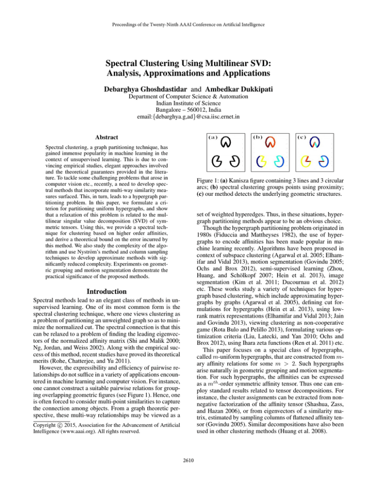
Figure 1: (a) Kanisza figure containing 3 lines and 3 circular
arcs; (b) spectral clustering groups points using proximity;
(c) our method detects the underlying geometric structures.
set of weighted hyperedges. Thus, in these situations, hypergraph partitioning methods appear to be an obvious choice.
Though the hypergraph partitioning problem originated in
1980s (Fiduccia and Mattheyses 1982), the use of hypergraphs to encode affinities has been made popular in machine learning recently. Algorithms have been proposed in
context of subspace clustering (Agarwal et al. 2005; Elhamifar and Vidal 2013), motion segmentation (Govindu 2005;
Ochs and Brox 2012), semi-supervised learning (Zhou,
Huang, and Schölkopf 2007; Hein et al. 2013), image
segmentation (Kim et al. 2011; Ducournau et al. 2012)
etc. These works study a variety of techniques for hypergraph based clustering, which include approximating hypergraphs by graphs (Agarwal et al. 2005), defining cut formulations for hypergraphs (Hein et al. 2013), using lowrank matrix representations (Elhamifar and Vidal 2013; Jain
and Govindu 2013), viewing clustering as non-cooperative
game (Rota Bulo and Pelillo 2013), formulating various optimization criteria (Liu, Latecki, and Yan 2010; Ochs and
Brox 2012), using Ihara zeta functions (Ren et al. 2011) etc.
This paper focuses on a special class of hypergraphs,
called m-uniform hypergraphs, that are constructed from mary affinity relations for some m > 2. Such hypergraphs
arise naturally in geometric grouping and motion segmentation. For such hypergraphs, the affinities can be expressed
as a mth -order symmetric affinity tensor. Thus one can employ standard results related to tensor decompositions. For
instance, the cluster assignments can be extracted from nonnegative factorization of the affinity tensor (Shashua, Zass,
and Hazan 2006), or from eigenvectors of a similarity matrix, estimated by sampling columns of flattened affinity tensor (Govindu 2005). Similar decompositions have also been
used in other clustering methods (Huang et al. 2008).
Introduction
Spectral methods lead to an elegant class of methods in unsupervised learning. One of its most common form is the
spectral clustering technique, where one views clustering as
a problem of partitioning an unweighted graph so as to minimize the normalized cut. The spectral connection is that this
can be relaxed to a problem of finding the leading eigenvectors of the normalized affinity matrix (Shi and Malik 2000;
Ng, Jordan, and Weiss 2002). Along with the empirical success of this method, recent studies have proved its theoretical
merits (Rohe, Chatterjee, and Yu 2011).
However, the expressibility and efficiency of pairwise relationships do not suffice in a variety of applications encountered in machine learning and computer vision. For instance,
one cannot construct a suitable pairwise relations for grouping overlapping geometric figures (see Figure 1). Hence, one
is often forced to consider multi-point similarities to capture
the connection among objects. From a graph theoretic perspective, these multi-way relationships may be viewed as a
c 2015, Association for the Advancement of Artificial
Copyright Intelligence (www.aaai.org). All rights reserved.
2610
In this paper, (1) we propose a method for partitioning
uniform hypergraphs by maximizing the squared associativity of the partition, and show that a relaxation of this problem is related to multilinear SVD of tensors (De Lathauwer,
De Moor, and Vandewalle 2000). (2) We use matrix perturbation analysis to provide theoretical bounds on the fraction
of data misclustered by the proposed algorithm. Next, (3)
we focus on the complexity of the algorithm, and develop
techniques for approximating the tensor decomposition using linear-time SVD (Drineas, Kannan, and Mahoney 2006)
and the Nyström approximation (Fowlkes et al. 2004). This
leads to a significant reduction of running time of the algorithm. (4) Experiments on geometric grouping and motion
segmentation show the practical importance of our method.
symmetric affinity matrix, and maximization of (1) is an alternative to the normalized associativity problem (Shi and
Malik 2000). We conclude this section by defining an operation for tensors that will be used in subsequent discussions.
Definition 2. Let A ∈ Rn1 ×n2 ×...×nm and U ∈ Rp×nk .
The mode-k product of A and U is a mth -order tensor, denoted by A ×k U ∈ Rn1 ×...nk−1 ×p×nk+1 ×...nm , such that
(A ×k U )i1 ...ik−1 jik+1 ...im =
Uniform hypergraph partitioning algorithm
We begin with mathematically formulating the problem of
maximizing squared associativity. For this, we follow the
approach used in case of graphs. Let H ∈ Rn×k such that
Hij = |Cj |−1/2 if vi ∈ Cj , and zero otherwise. Using the
definition of mode-k product, one can write the maximization of (1) as the following optimization:
Tensors and Uniform hypergraphs
maximize
Ci ,...,Ck
k
X
W ×1 hTj ×2 hTj . . . ×m hTj
2
,
(2)
j=1
where hj denotes the j th column of H. Note that h1 , . . . , hk
are orthonormal. However, the above problem is hard. So we
relax it by allowing H ∈ Rn×k to be any matrix with orthonormal columns. At this stage, we rely on the multilinear
SVD of symmetric tensors. The following theorem summarizes a number of results in (De Lathauwer, De Moor, and
Vandewalle 2000; Chen and Saad 2009).
Theorem 3. Let W be a mth -order n-dimensional symmetric tensor. Then the solution to the problem
Since the hypergraph is undirected, the tensor W is symmetric, i.e., for any permutation σ of indices, we have
Wi1 i2 ...im = Wiσ(1) iσ(2) ...iσ(m) for all tuples (i1 i2 . . . im ).
For partitioning the hypergraph, we need a notion of total
similarity of any group of vertices. We define this in terms
of the associativity, as described below.
Definition 1. Let C ⊂ V be a group of vertices. The associativity of C is defined as
X
Assoc(C) =
Wi1 i2 ...im .
maximize
U ∈Rn×k :U T U =I
k
X
W ×1 uTj ×2 uTj . . . ×m uTj
2
j=1
is the matrix U containing the k leading orthonormal left
c ∈ Rn×nm−1 , given by
singular vectors of the matrix, W
cij = Wii ...i
W
2
m
when j = 1 +
m
X
(il − 1)nl−2 . (3)
l=2
vi1 ,vi2 ,...,vim ∈C
n×(n−k)
Furthermore, if Ũ ∈ R
contains the remaining left
c
singular vectors of W , then one can express W as
In addition, for a partition C1 , . . . , Ck of V, we define the
squared associativity of the partition as
k
X
(Assoc(Cj ))2
j=1
Ai1 ...ik−1 ik ik+1 ...im Ujik .
ik =1
The problem at hand is that of grouping n given objects,
V = {v1 , . . . , vn }, into k disjoint clusters, C1 , . . . , Ck . A
weighted undirected m-uniform hypergraph H on V is a
triplet H = (V, E, w), where V is a set of vertices and E
is the set of hyperedges, with each hyperedge being a collection of m vertices. The function w : E → R assigns a
real-valued weight to each hyperedge. Our primary aim for
constructing a hypergraph is to capture the similarity among
m-tuples of vertices (data points), which are used to partition V into the k disjoints sets.
One can represent the affinities of a m-uniform hypergraph by a mth -order W ∈ Rn×n×...×n such that
w(e) if ∃e ∈ E, e = {vi1 , ..., vim },
Wi1 i2 ...im =
0
otherwise.
SqAssoc(C1 , . . . , Ck ) =
nk
X
|Cj |m
W = Σ ×1 [U Ũ ] ×2 . . . ×m [U Ũ ],
,
(1)
(4)
Σ being a mth -order n-dimensional all-orthogonal tensor.
The decomposition in (4) is known as the multilinear SVD
of symmetric tensors. The above result states that the solution to the relaxed partitioning problem is given by the left
c corresponding to the largest singusingular vectors of W
lar values. One can also think of the optimizer U as the k
cW
c T . Based on
leading orthonormal eigenvector matrix of W
this, we propose the algorithm that is listed as Algorithm 1.
The primary reason for clustering the rows of U is as follows: U acts as an approximation of the matrix H in (2) for
which the rows corresponding to vertices in same cluster are
where |C| denotes the number of vertices in cluster C.
Though the above definition looks similar to association
score of kernel k-means (Zha et al. 2001), it is significantly
different as it incorporates multi-way affinities, and it does
not correspond to a Euclidean norm minimization as in kmeans. In the next section, we formulate an approach that
partitions the hypergraph by maximizing (1), and relax it
to obtain a spectral algorithm. For undirected graphs (2uniform hypergraphs), the above discussion holds for the
2611
Algorithm 1 Clustering using m-ary affinity relations
1. thereexists > 0 such that size of each cluster is at least
max n
,
2m
−
1
,
qk
m−2
2. n ≥ 2(m − 1) 2k
, and
− 2k + 2
T
cW
cT − W
d∗ W
d∗ k2 ≤ 1 m nm-α for some α > 0
3. kW
16 2k
where k · k2 is matrix operator norm. Then the fraction of
nodes, misclustered by Algorithm 1 is at most kn−2α .
th
Given: An m -order affinity tensor W that contains the mary affinity relations among objects V = {v1 , . . . , vn }.
c from W using (3).
1. Construct W
2. Let U ∈ Rn×k be the matrix of k leading orthonormal
c (or eigenvectors of W
cW
c T ).
left singular vectors of W
3. Cluster the rows of U into k clusters using k-means, and
partition V accordingly.
T
d∗ W
d∗
Proof. Due to the form of W∗ (5), the matrix W
has a block diagonal structure when the vertices are ordered
according to the true partition. Here, each non-zero block
corresponds to each cluster. The eigen-gap, δ, between the
T
d∗ W
d∗ can be
k th and (k + 1)th largest eigenvalues of W
bounded below as (Chen and Lerman 2009, Proposition 4.8)
m−2
m
n m
δ ≥ 2k
≥ 12 2k
− (m − 1) n − k−1
(6)
n
k n
where the first inequality uses condition 1, and the second
relies on condition 2 of the proposition. From condition 3
and Weyl’s inequality, the absolute difference between the
T
cW
c T and W
d∗ W
d∗ is bounded
ith largest eigenvalues
of W
m
1
above by 16
nm-α < 2δ for all i = 1, . . . , n. Based on
2k
this, we use the Davis-Kahan perturbation theorem to claim
the following: If U, U ∗ ∈ Rn×k are matrices of k leading
T
cW
c T and W
d∗ W
d∗ , respecorthonormal eigenvectors of W
tively, then there is a rotation matrix O ∈ Rk×k such that
identical. Hence, it must hold approximately for U also. A
more concrete justification is presented in the next section.
One can observe the resemblance of Algorithm 1 with the
spectral clustering algorithm (Ng, Jordan, and Weiss 2002).
The method in (Govindu 2005) is also similar to Algorithm 1, but includes certain additional steps such as normalcW
c T , and approximation of the tensor. Moreization of W
over, the method in (Govindu 2005) does not arise from a
hypergraph partitioning formulation.
Perturbation analysis of proposed method
We now study the theoretical validity of the above approach.
Formally, we derive an upper bound on the error made by
Algorithm 1. The subsequent discussion is based on matrix
perturbation analysis, which has been often used to analyze
spectral techniques. Error bounds for spectral clustering using perturbation analysis have been studied in (Ng, Jordan,
and Weiss 2002; Rohe, Chatterjee, and Yu 2011). Chen and
Lerman (2009) used similar techniques to analyze an approach similar to (Govindu 2005), while Ghoshdastidar and
Dukkipati (2014) used perturbation bounds to provide similar guarantees in a semi-random setting.
The idea of perturbation analysis is to study the method
in an ideal case, and then provide bounds by considering the
affinity relations in the general case as a perturbation of the
ideal scenario. In the ideal case, we assume that the partition
is known and there is a hyperedge of unit weight on a set of
m distinct vertices only when all the vertices belong to the
same cluster. So the ideal affinity tensor is given as
(
1 if i1 , . . . , im , are distinct and
∗
vi1 , ..., vim ∈ Cj for some j,
Wi1 i2 ...im =
(5)
0 otherwise.
T
cW
cT − W
d∗ W
d∗ k2
1
2kW
2
≤ 2α , (7)
kU − U
≤
2
(δ/2)
8n
where the last inequality follows from (6) and condition
3. We can combine this with the fact kU − U ∗ Ok2F ≤
kkU − U ∗ Ok22 to obtain a bound on Frobenius norm. Moreover, since δ > 0, one can see that U ∗ has exactly k distinct
rows, each corresponding to a particular cluster.
Assume that the k-means step in Algorithm 1 achieves its
global optimum. Let ci ∈ Rk denote the k-means centroid
corresponding to the ith data instance, and c∗i ∈ Rk be the
ith row of U ∗ O. It is observed in (Rohe, Chatterjee,
and Yu
√
2011, Lemma 3.2) that if kci − c∗i k < 1/ 2nmax , then the
ith node is correctly clustered. Here, nmax is the maximum
cluster size which is bounded as nmax ≤ (1− k−1
k )n. Thus,
the number of misclustered nodes is bounded
by the num√
ber of nodes for which kci − c∗i k ≥ 1/ 2nmax , which can
be in turn bounded using the fact that ci ’s are obtained by
minimizing objective of k-means algorithms. So, we have
fraction of misclustered √
nodes
|{i : kci − c∗i k ≥ 1/ 2nmax }|
8nmax kU − U ∗ Ok2F
≤
≤
n
n
which can be bounded using (7) to arrive at the claim.
∗
A similar tensor has been used in (Chen and Lerman 2009),
and the performance of the algorithm using such tensor can
be found in (Chen and Lerman 2009, Proposition 4.8). However, while studying the general case, we deviate from the
analysis in (Chen and Lerman 2009), and use a variant of
the Davis-Kahan sin Θ theorem (Rohe, Chatterjee, and Yu
2011) which helps us to bound the fraction of misclustered
nodes, thereby providing a more useful result. The analysis
of Algorithm 1 is summarized in the following proposition.
Proposition 4. let W be an mth -order n-dimensional affinity tensor of a hypergraph with k partitions, W∗ be the corc, W
d∗ be their respecresponding ideal affinity tensor and W
tive flattened matrices. Let the following conditions hold:
Ok22
The above result implies that as n increases, if the conditions hold for some fixed α > 0, then the fraction of
misclustered nodes goes to zero. Hence, Algorithm 1 provides accurate clustering as the sample size increases. The
use of operator norm helps to obtain a less strict assumption
in condition 3, as compared to the Frobenius norm considered in (Rohe, Chatterjee, and Yu 2011; Ghoshdastidar and
Dukkipati 2014).
2612
Complexity and approximations
hence, uninformative. Reducing the rejection can be possible in certain problems as motion segmentation and subspace clustering by choosing vertices that are in close proximity or closely define a subspace. This can be achieved by
performing an initial run of k-means or k-subspaces (Ho et
al. 2003) algorithms. However, the number of initial clusters
required depends on the nature of problem at hand. One can
derive error bounds for above method by combing Proposition 4 with (Drineas, Kannan, and Mahoney 2006, Theorem 4). The method of rejecting columns of small magnitude
is essential to achieve reasonable bounds.
While the previous section shows that the Algorithm 1 is accurate for large sample size, the complexity of the method
(in its crude form) is as large as O(nm+1 ). This is mainly
due to the large number of computations required to compute all the entries of the tensor. In this section, we study
some techniques to determine the eigenvector matrix U by
sampling elements of the tensor. This significantly reduces
the complexity as one only needs to compute values of
the sampled entries. Our discussion is based on two popular sampling techniques for matrices, namely column sampling (Drineas, Kannan, and Mahoney 2006) and Nyström
approximation (Fowlkes et al. 2004). In the latter case, we
generalize the existing approach to the case of symmetric
tensors. We also discuss a simple technique to extend the
clustering to a large number of unsampled entries.
Nyström approximation
This method approximates the eigen-decomposition of symmetric matrices using only a sampled set of entries (Fowlkes
et al. 2004; Drineas and Mahoney 2005). One randomly
samples c columns of the matrix, and computes the k leading eigenvectors of the matrix formed by intersection of the
sampled c columns with corresponding c rows. The Nyström
extension of the above eigenvectors are then computed using other entries of the sampled columns. The key observation at this stage lies in the fact that the Nyström extension
of eigenvectors is such that, if k = c, then the c sampled
columns of the original matrix are accurately reproduced in
the Nyström approximation of the matrix. Using this fact,
we present a similar method for symmetric tensors.
Suppose we have a mth -order n-dimensional symmetric tensor W. We focus on an approximate decomposition
similar to the one in (4) (Proposition 3), with time complexity significantly less than O(nm+1 ). Following the strategy of Nyström’s method, we sample a mth -order subtensor
A ∈ Rr×...×r , which contains m-way affinities of r sampled vertices. Let the multilinear SVD of A be given by
Column sampling and Linear-time SVD
We recall that our primary interest is to compute the k leadc ∈ Rn×nm−1 . We
ing left singular vectors of the matrix W
can solve this using the linear-time SVD algorithm (Drineas,
Kannan, and Mahoney 2006), which uses only some c number of sampled columns to compute an approximate SVD.
However, this approach requires to read the matrix once
from an external storage to determine the probabilities for
sampling each column. Since, this process is extremely
costly in our case, we use a variation of linear-time SVD.
Below, we state the modification of Algorithm 1 combined
c
with this approximation. Note here that each column of W
corresponds to fixing (m − 1) vertices, while the entries are
computed by varying the mth vertex.
Algorithm 2 Column sampling variant of Algorithm 1
Given: An m-way affinity measure among {v1 , . . . , vn };
Number of sampled columns c; Threshold parameter τ > 0.
1. Compute a matrix C ∈ Rn×c as follows:
For t = 1 to c
(a) Randomly select (m − 1) vertices.
(b) Compute w ∈ Rn whose entries are m-way affinities
of all vertices with (m − 1) chosen vertices.
(c) If kwk < τ , goto 1(a), else set tth column of C as w.
2. Let U be the matrix of k leading left eigenvectors of C.
3. Cluster the rows of U into k clusters using k-means, and
partition V accordingly.
A = Σ1 ×1 U1 ×2 U1 ×3 . . . ×m U1 ,
(8)
b the
where U1 ∈ Rr×r is the left singular vector matrix of A,
flattening matrix of A.
Next, we compute an extension of U1 in a spirit similar
to that of Nyström extension, i.e., by closely approximating
the affinities among sampled and unsampled instances. In
the case of matrices, we require only O(r(n − r)) memory
to represent all such affinities. However, in case of m-way
affinity, the number of possible entries is (n−r)rnm−2 considering all the cases where affinity is constructed over a set
of size m that includes at least one sampled and one unsampled instance. To avoid such high memory requirement, we
use only the m-way affinities defined over one unsampled
instance and (m − 1) of the sampled points. This can be represented in a mth -order tensor B ∈ R(n−r)×r×...×r , whose
first index varies over all unsampled data instances and the
rest over the r sampled instances.
Let U2 ∈ R(n−r)×r be an extension of the eigenvectors
to the unsampled instances. Using this, we may write the
approximation of the tensor W as
U1
U1
f
W = Σ1 ×1
×2 . . . ×m
.
(9)
U2
U2
nc
The above algorithm can be performed in O( 1−η
+ kn2 ),
where η is the rate of rejecting columns in Step 1(c).
Govindu (2005) also used a column sampling heuristic, but
did not consider rejecting columns. Rejection is essential
because of the following reason. Consider the line clustering problem stated in the introduction. Here, any column
c contains useful information only if the correspondof W
ing (m − 1) vertices belong to the same cluster. Otherwise,
all the entries in the column contain small values, and it is
2613
Our objective here is to find U2 such that we can approxif then
mate the subtensor B well in (9). Note, if W ≈ W
B ≈ Σ1 ×1 U2 ×2 U1 . . . ×m U1 = A ×1 U2 U1T ,
(10)
where we use (8) to simplify the expression. However,
this may not be achieved in general because (10) imposes
rm−1 (n − r) conditions, while there are only r(n − r) variables in U2 . Hence, we opt for a least squares solution, where
we minimize the k·kF -norm of the difference of the two tensors. This norm is defined similar to the Frobenius norm of
matrices, i.e., k · k2F denotes the sum of squares of all entries of a tensor. The solution to this problem is given in the
following result.
Proposition 5. Let A, B and U1 be as above. Then
2
U2 = arg min B − A ×1 ZU1T Algorithm 3 Nyström approximation of Algorithm 1
Given: An m-way affinity measure among {v1 , . . . , vn };
Number of initial clusters kr ; Number of vertices chosen
from each cluster nr (≥ (m − 1)).
1. Form initial kr clusters using k-means or k-subspaces.
2. From each cluster, randomly sample nr data instances to
form the set of r = nr kr vertices.
3. Compute the mth -order affinity tensor, A, for the sampled vertices, and compute U1 ∈ Rr×k , the k leading left
b
singular vector matrix of A.
4. Compute B as describe above.
5. Find the Nyström extension U ∈ Rn×k using (11), and
orthonormalize its columns.
6. Cluster the rows of U into k clusters using k-means, and
partition V accordingly.
F
Z∈R(n−r)×r
−1
bA
bT U1 U1T A
bA
bT U1
=B
,
b ∈ Rr×rm−1 and B
b ∈ R(n−r)×rm−1 are obtained
where A
from A and B, respectively, by flattening (3). Thus, the
Nyström extension of U1 is given by
!
U1
−1
U=
.
(11)
bA
bT U1 U T A
bA
bT U1
B
Extending labels by fitting
Often in problems such as subspace clustering and geometric grouping, each cluster represents a geometric object, and
the m-way affinities are computed based on the error of fitting m points in such a model. For these problems, one can
often work on a sampled set of data instances. Provided that
the clusters are accurately detected on this sampled set, one
can easily extend the clustering result to other unsampled
data points by the following procedure.
1
Proof. The key in this proof is to appropriately express the
the norm k · kF for tensor in terms of the corresponding flattened matrix. One can verify that
b − ZU1T Ak
b 2F ,
B − A ×1 ZU1T 2 = kB
1. For each of the k obtained clusters, fit a model based on
the data assigned to the cluster.
F
the latter being the standard Frobenius norm for matrices.
The minimizer U2 of the above problem satisfies
bA
bT U1 = U2 U1T A
bA
bT U1 ,
B
2. For each new sample, compute the fitting error for each of
the k models, and assign it to the cluster for which fitting
error is least.
and hence, the claim.
This approach runs in linear time, but requires a good initial
labeling to start with. Hence, we recommend this approach
only when the data is considerably large, and a small fraction
of data can be accurately clustered using Algorithms 2 or 3.
bA
bT U1 is diagonal with nonWe note that the matrix U1T A
negative entries. Hence, one can simply use the pseudoinverse in case some diagonal entries are zero. Moreover, we
are interested in only the k leading orthonormal eigenvectors. This can be simply obtained by selecting the k leading
eigenvectors in U1 , and orthonormalize the corresponding
columns of Nyström extension.
One requires to choose the r vertices wisely. For this, we
use the idea in (Zhang, Tsang, and Kwok 2008), where the
authors suggest an initial k-means clustering to select the r
landmark points, which are centers of k clusters. However,
in our case, it is more appropriate to perform an initial kmeans or k-subspaces clustering and choose at least (m − 1)
points from each cluster as one requires expects high m-way
affinity for other points in same cluster with a chosen collection of points. The intuition for effectiveness for initial
k-means clustering is that in a number of subspace clustering or motion segmentation problems, closely located data
instances often lie in same cluster. Based on this, we present
Algorithm 3 which has O(rm+1 +kr2 +knrm−1 ) time complexity, where r = nr kr , kr being the initial number of clusters and nr the number of points chosen from each cluster.
Experimental validation
In this section, we conduct experiments on geometric grouping and motion segmentation. Figure 1 in introduction shows
that one cannot group geometric objects using pairwise
affinities. Hence, one requires higher order similarities based
on error on fitting geometric models. In such problems, we
choose a geometric structure, and for any set of m points,
we compute the error (f ) of fitting these points into the assumed model. The m-way affinity is simply e−cf for some
parameter c > 0. Note that one has to choose m larger
than the number points that uniquely define the model. A
suitable choice is m = 3 for line fitting, and m = 4
for circle and plane fitting. The sample size (n) and the
tensor order (m) in Figure 2 show that the computational
time required to work with the complete tensor is difficult
in such cases, and so the works in (Agarwal et al. 2005;
Zhou, Huang, and Schölkopf 2007; Rota Bulo and Pelillo
2013) etc. cannot be used. Hence, approximate methods
2614
Finally, we conduct experiments on the Hopkins 155 motion segmentation database (Tron and Vidal 2007), where
each video contains two or three independent motions. There
are 120 videos with two motions, and 35 videos with three
motions. It is well known that trajectories of each rigid motion span a low-dimensional subspace. For each problem,
we use 4th -order tensors, and fit group of four trajectories
in a subspace of dimension 2. The affinities are of the form
e−cf (·) , where f (·) is the fitting error. Table 1 reports the
mean and median percentage error of clustering computed
for all datasets with 2 or 3 motions. The table compares our
method with 7 existing approaches for motion segmentation.
The results in top six rows have been taken from (Jain and
Govindu 2013). The results in Table 1 clearly show that our
method achieves almost best performance in case of 2 motion problems. For 3 motion segmentation, the mean error
is worse than LRR-H, SSC and SGC, but the median of
the errors is better than these. Overall, though SGC (Jain
and Govindu 2013) gives best performance on Hopkins 155
database, our approach achieves almost similar accuracy. We
also note that an initial clustering before sampling helps to
significantly reduce the error compared to (Govindu 2005).
such as Algorithms 2 and 3 are required. Figure 2 (right
column) clearly shows that these approximation techniques
work quite well in such problems. Moreover, in case of the
second problem in Figure 2, even approximate methods require significant time. So we use only 1% of the data and
extend the labeling by the method of fitting discussed above.
Clustering
edge pixels
n = 1047
k=9
m=3
Detected edges
Clustered edges
Depth map
Clustered faces
Clustering
cube faces
n = 38726
k=3
m=4
Figure 2: Geometric grouping using proposed method.
Method
2 motions
3 motions
All videos
Mean Median Mean Median Mean Median
To give an experimental comparison of the two proposed
approximation methods, we consider a problem of grouping
points on three randomly generated intersecting lines using
3rd order affinities based on line fitting error. In this case, using the entire affinity tensor is similar to the ideal case, and
hence, the leading eigenvectors are indicators of the true assignments. In Figure 3, we compare the errors incurred and
time taken by Algorithms 2 and 3 as the fraction of entries
sampled from the tensor increases. The error is measured in
terms of difference in the subspaces spanned by the leading orthonormal eigenvectors of the entire tensor and the approximate eigenvectors computed by the Algorithms. This
difference can be computed as in (Rohe, Chatterjee, and Yu
2011, Appendix B). Figure 3 clearly shows that when less
entries are sampled, column sampling gives better approximation. But, as sampling increases error incurred by both
methods are quite similar. This shows that the variation of
similarities over the entire data is not captured well when
less samples are used in Nyström approximation. On the
other hand, for higher number of samples, column sampling
requires more time due to rejection of columns.
LSA
SCC
LRR
LRR-H
LRSC
SSC
SGC
Govindu
Ours
4.23
2.89
4.10
2.13
3.69
1.52
1.03
1.83
1.05
0.56
0.00
0.22
0.00
0.29
0.00
0.00
0.00
0.00
7.02
8.25
9.89
4.03
7.69
4.40
5.53
9.31
5.72
1.45
0.24
6.22
1.43
3.80
0.56
0.35
5.71
0.28
4.86
4.10
5.41
2.56
4.59
2.18
2.05
3.52
2.11
0.89
0.00
0.53
0.00
0.60
0.00
0.00
0.03
0.00
Table 1: Mean and median of percentage error incurred by
different algorithms on the Hopkins 155 dataset.
Conclusion
In this paper, we studied an extension of spectral clustering
to the case of uniform hypergraphs. We formulated the problem of maximizing squared associativity of uniform hyper
graphs, and showed that a relaxation of this problem is related to the multilinear SVD of the affinity tensor of the hypergraph. Based on this, we proposed a spectral hypergraph
partitioning algorithm, and derived a theoretical bound for
the fractional error incurred by the algorithm. We also developed approximation techniques to reduce the time complexity of the algorithm using linear-time SVD and Nyström’s
method, and experimentally compared these two approximations. We also demonstrated the accuracy of the proposed
algorithm in geometric grouping and motion segmentation.
Acknowledgement
Figure 3: (left) Error incurred and (right) time taken by Algorithms 2 and 3 as the number of sampled entries varies.
Black line is for Algorithm 2 and red line for Algorithm 3.
The authors would like to thank the reviewers for suggesting important references. D. Ghoshdastidar is supported by
Google Ph.D. Fellowship in Statistical Learning Theory.
2615
References
high order svd and k-means clustering. In Proceedings of the
14th ACM SIGKDD international conference on Knowledge
Discovery and Data mining, 327–335.
Jain, S., and Govindu, V. M. 2013. Efficient higher-order
clustering on the grassmann manifold. In IEEE International Conference on Computer Vision.
Kim, S.; Nowozin, S.; Kohli, P.; and Yoo, C. D. 2011.
Higher-order correlation clustering for image segmentation.
In Advances in Neural Information Processing Systems.
Liu, H.; Latecki, L. J.; and Yan, S. 2010. Robust clustering
as ensembles of affinity relations. In Advances in Neural
Information Processing Systems, 1414–1422.
Ng, A.; Jordan, M.; and Weiss, Y. 2002. On spectral clustering: analysis and an algorithm. In Advances in Neural
Information Processing Systems, 849–856.
Ochs, P., and Brox, T. 2012. Higher order motion models
and spectral clustering. In Proceedings of the IEEE Conference on Computer Vision and Pattern Recognition.
Ren, P.; Aleksić, T.; Wilson, R. C.; and Hancock, E. R.
2011. A polynomial characterization of hypergraphs using
the ihara zeta function. Pattern Recognition 44(9):1941–
1957.
Rohe, K.; Chatterjee, S.; and Yu, B. 2011. Spectral clustering and the high-dimensional stochastic blockmodel. Annals
of Statistics 39(4):1878–1915.
Rota Bulo, S., and Pelillo, M. 2013. A game-theoretic approach to hypergraph clustering. IEEE Transactions on Pattern Analysis and Machine Intelligence 35(6):1312–1327.
Shashua, A.; Zass, R.; and Hazan, T. 2006. Multi-way clustering using super-symmetric non-negative tensor factorization. In European Conference on Computer Vision, 595–
608.
Shi, J., and Malik, J. 2000. Normalized cuts and image
segmentation. IEEE Transactions on Pattern Analysis and
Machine Intelligence 22(8):888–905.
Tron, R., and Vidal, R. 2007. A benchmark for the comparison of 3-d motion segmentation algorithms. In Proceedings of the IEEE Conference on Computer Vision and Pattern Recognition.
Zha, H.; He, X.; Ding, C.; Simon, H.; and Gu, M. 2001.
Spectral relaxation for k-means clustering. In Advances in
Neural Information Processing Systems.
Zhang, K.; Tsang, I. W.; and Kwok, J. T. 2008. Improved
Nyström low-rank approximation and error analysis. In Proceedings of the International Conference on Machine Learning.
Zhou, D.; Huang, J.; and Schölkopf, B. 2007. Learning with
hypergraphs: Clustering, classification, and embedding. In
Advances in Neural Information Processing Systems, 1601–
1608.
Agarwal, S.; Lim, J.; Zelnik-Manor, L.; Perona, P.; Kriegman, D.; and Belongie, S. 2005. Beyond pairwise clustering. In IEEE Conference on Computer Vision and Pattern
Recognition, 838–845.
Chen, G., and Lerman, G. 2009. Foundations of a multi-way
spectral clustering framework for hybrid linear modeling.
Foundations of Computational Mathematics 9:517–558.
Chen, J., and Saad, Y. 2009. On the tensor SVD and the optimal low rank orthogonal approximation of tensors. SIAM
Journal on Matrix Analysis and Applications 30(4):1709–
1734.
De Lathauwer, L.; De Moor, B.; and Vandewalle, J. 2000.
A multilinear singular value decomposition. SIAM Journal
on Matrix Analysis and Applications 21(4):1253–1278.
Drineas, P., and Mahoney, M. W. 2005. On the nyström
method for approximating a Gram matrix for improved
kernel-based learning. Journal of Machine Learning Research 6:2153–2175.
Drineas, P.; Kannan, R.; and Mahoney, M. W. 2006. Fast
Monte Carlo algorithms for matrices II: Computing a lowrank approximation to a matrix. SIAM Journal of Computing
36(1):158–183.
Ducournau, A.; Bretto, A.; Rital, S.; and Laget, B. 2012. A
reductive approach to hypergraph clustering: An application
to image segmentation. Pattern Recognition 45(7):2788–
2803.
Elhamifar, E., and Vidal, R. 2013. Sparse subspace clustering: Algorithm, theory, and applications. IEEE Transactions
on Pattern Analysis and Machine Intelligence 35(11).
Fiduccia, C. M., and Mattheyses, R. M. 1982. A linear-time
heuristic for improving network partitions. In 19th Design
Automation Conference, 175–181.
Fowlkes, C.; Belongie, S.; Chung, F.; and Malik, J. 2004.
Spectral grouping using the Nyström method. IEEE Trans.
on Pattern Analysis and Machine Intelligence 26(2):214–
225.
Ghoshdastidar, D., and Dukkipati, A. 2014. Consistency of
spectral partitioning of uniform hypergraphs under planted
partition model. In Advances in Neural Information Processing Systems.
Govindu, V. M. 2005. A tensor decomposition for geometric grouping and segmentation. In IEEE Computer Society
Conference on Computer Vision and Pattern Recognition,
1150–1157.
Hein, M.; Setzer, S.; Jost, L.; and Rangapuram, S. 2013. The
total variation on hypergraphs-learning on hypergraphs revisited. In Advances in Neural Information Processing Systems, 2427–2435.
Ho, J.; Yang, M.-H.; Lim, J.; Lee, K.-C.; and Kriegman, D.
2003. Clustering appearances of objects under varying illumination conditions. In Proceedings of the IEEE Conference
on Computer Vision and Pattern Recognition.
Huang, H.; Ding, C.; Luo, D.; and Li, T. 2008. Simultaneous
tensor subspace selection and clustering: the equivalence of
2616