Proceedings of the Thirtieth AAAI Conference on Artificial Intelligence (AAAI-16)
Generalised Brown Clustering and Roll-Up Feature Generation
Leon Derczynski
Sean Chester
University of Sheffield
211 Portobello, Sheffield S1 4DP
United Kingdom
leon@dcs.shef.ac.uk
NTNU Aarhus Universitet
Sem Saelandsvei 9 Åbogade 34
7491 Trondheim, Norway 8200 Aarhus N, Denmark
sean.chester@idi.ntnu.no
Abstract
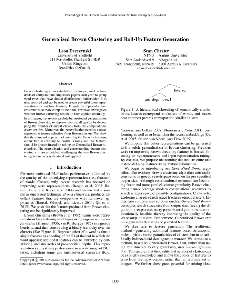
love, eat
Brown clustering is an established technique, used in hundreds of computational linguistics papers each year, to group
word types that have similar distributional information. It is
unsupervised and can be used to create powerful word representations for machine learning. Despite its improbable success relative to more complex methods, few have investigated
whether Brown clustering has really been applied optimally.
In this paper, we present a subtle but profound generalisation
of Brown clustering to improve the overall quality by decoupling the number of output classes from the computational
active set size. Moreover, the generalisation permits a novel
approach to feature selection from Brown clusters: We show
that the standard approach of shearing the Brown clustering
output tree at arbitrary bitlengths is lossy and that features
should be chosen insead by rolling up Generalised Brown hierarchies. The generalisation and corresponding feature generation is more principled, challenging the way Brown clustering is currently understood and applied.
1
cats, dogs you, I
Figure 1: A hierarchical clustering of semantically similar
terms. Leaves correspond to clusters of words, and leaves
near common parents correspond to similar clusters.
Carreras, and Collins 2008; Blunsom and Cohn 2011), performing as well as or better than the recent embeddings (Qu
et al. 2015; Šuster, van Noord, and Titov 2015).
We propose that better representations can be generated
with a subtle generalisation of Brown clustering. Previous
work on improving Brown clustering features is limited, focusing on hyperparametre and input representation tuning.
By contrast, we propose abandoning the tree structure and
instead defining features using mutual information.
We begin by introducing our Generalised Brown algorithm. The existing Brown clustering algorithm artificially
constrains its greedy search space based on the pre-specified
output size. Although computational resources are becoming faster and more parallel, coarse granularity Brown clustering cannot leverage modern computational resources to
search a larger space of possible configurations. Conversely,
exploring a larger search space fractures output clusters. Either case compromises solution quality. Generalised Brown
decouples search space size from output size, freeing the algorithm to explore as many possible configurations as computationally feasible, thereby improving the quality of the
set of output clusters. Furthermore, Generalised Brown run
once generates thousands of potential features.
We then turn to feature generation. The traditional
method—generating additional features based on ancestor
nodes—yields varied granularities of clusters, but in an artificially balanced and data-agnostic manner. We introduce a
method, based on Generalised Brown, that, rather than using tree structure to vary granularity, uses mutual information. This ensures that the quality and number of clusters can
be explicitly controlled, and allows the choice of features to
arise from the input corpus, rather than an arbitrary set of
integers. We further show great potential for mining ideal
Introduction
For most statistical NLP tasks, performance is limited by
the quality of the underlying representation (i.e., features)
of words. Consequently, recent research has focused on
improving word representations (Bengio et al. 2003; Baroni, Dinu, and Kruszewski 2014) and shown that a simple unsupervised technique, Brown clustering, produces excellent features that are competitive with far newer approaches (Bansal, Gimpel, and Livescu 2014; Qu et al.
2015). We posit that the features produced from Brown clustering can be significantly improved.
Brown clustering (Brown et al. 1992) learns word representations by clustering word types using bigram mutual information (Shannon 1956; van Rijsbergen 1977) as a greedy
heuristic, and then constructing a binary hierarchy over the
clusters (like Figure 1). Representation of a word is thus a
single feature: an encoding of the ID of the leaf in which the
word appears; additional features can be extracted by considering ancestor nodes at pre-specified depths. This representation yields strong performance in a wide range of NLP
tasks, including semi- and unsupervised scenarios (Koo,
c 2016, Association for the Advancement of Artificial
Copyright Intelligence (www.aaai.org). All rights reserved.
1533
Cluster ID
00111001
001011111001
01111010111110
Figure 1). The use of mutual information as a greedy heuristic produces clusters wherein member word types are found
in similar contexts (i.e. have similar distributionality). Paths
to clusters are given as bit strings, indicating branches from
the root. Table 1 shows some example Brown clusters from
a large corpus.
Constituent word types
can cn cann caan cannn ckan shalll
ccan caaan cannnn caaaan
ii id ion iv ll iii ud wd uma ul idnt
provoking hed 1+1 ididnt hast ine
2+2 idw #thingsblackpeopledo iiii
#onlywhitepeople dost doan
uon apt-get
hoping wishing considering wishin
contemplating dreading regretting
hopin hopeing considerin
suspecting regreting wishn
comtemplating hopen
Notation We first introduce the following notation. Let S
denote an input sequence and let VS denote the unique symbols in sequence S (i.e., the vocabulary), sorted by descending frequency.2 By VS [k], we denote the k’th symbol in VS .
A cluster, Ci , is a subset of VS and all clusters are disjoint
(i.e., Ci ∩ Cj = ∅ =⇒ i = j). A complete
clustering of the
vocabulary is a set
of
clusters
C
=
C
,
.
.
. , C|C|−1 that
0
is complete (i.e., Ci = VS ). Also, adjacent symbols (i.e.,
bigrams) in S are denoted l, r and the relative frequency
of l, r in S is denoted p(l, r).
Further, let p(l, ∗) =
r∈V(S) p(l, r) and p(∗, r) =
l∈V(S) p(l, r).
Analogously,
we denote adjacent symbols from Ci and Cj
by Ci , Cj = l∈Ci ,r∈Cj l, r, and the relative frequency
in
Finally, let p(Ci , ∗) =
S of Ci , Cj as p(Ci , Cj ). l∈Ci p(l, ∗) and p(∗, Cj ) =
r∈Cj p(∗, r).
The average mutual information (AMI) of a set of clusters is defined in two parts (Definitions 1-2). AMI is high if
frequent bigrams appear nearly as often as their two symbols
independently appear:
Table 1: Sample Brown clusters over English tweets.1
features from the Generalised Brown output.
These contributions may profoundly change the way
Brown clustering is understood and employed. This alreadypowerful technique gains a strong overhaul as a result.
Outline and contributions Section 2 formally describes
Brown clustering and related work. Sections 3-4 present and
validate contributions, listed below. Section 5 concludes.
• We generalise the Brown clustering algorithm by introducing a new hyper-parametre, active set, a; we completely decouple the well-known hyper-parametre, number of classes, from computation (Section 3).
Definition 1 (Mutual information/MI). The mutual information of two classes, Ci , Cj ∈ C, denoted MI(Ci , Cj ), is3 :
MI(Ci , Cj ) = p(Ci , Cj ) log2
• Based on Generalised Brown, we introduce a new method
of feature selection that varies granularity based on mutual information, rather than hierarchical path length, improving down-stream NER performance (Section 4).
p(Ci , Cj )
p(Ci , ∗) p(∗, Cj )
Definition 2 (Average mutual information/AMI). The average mutual information of C, denoted AMI(C), is the sum
of mutual information of all pairs of clusters in C:
MI(Ci , Cj )
AMI(C) =
• We release a software toolkit for creating the generalised
output and feature extraction we present.
Ci ,Cj ∈C
2
The classic view of Brown clustering
The Brown clustering algorithm repeatedly finds from a
set of clusters a top pair (Definition 4) based on AMI and
then conducts a merge (Definition 3) of the top pair.
We begin by re-presenting Brown clustering for both the
familiar and unfamiliar reader, for two reasons. First, we
favour a more formal definition of the algorithm than was
presented originally (Brown et al. 1992) and in subsequent
work. Second, our presentation of Brown clustering will better illuminate the changes in our generalisation thereof.
We present first the clustering algorithm and notation used
throughout this paper (Section 2.1), then methods for extracting features from the algorithm’s output (Section 2.2).
2.1
Definition 3 (Merge). A merge operation in C, denoted
Ci←j combines clusters Ci and Cj :
Ci←j = (C \ {Ci , Cj }) ∪ {Ci ∪ Cj }
Definition 4 (Top pair). A top pair, denoted π̂(C), is a pair
of classes the merging of which least reduces AMI:
π̂(C) = arg max
The clustering method, formalised
Ci ,Cj ∈C,i=j
Brown clustering (Brown et al. 1992) is a greedy, hierarchical, agglomerative hard clustering algorithm to partition a
vocabulary into a set of clusters with minimal loss in mutual information (Shannon 1956; van Rijsbergen 1977). The
target number of clusters is specified in advance and these
output clusters are organised as leaves of a binary tree (as in
Algorithm description Algorithm 1 describes Brown
clustering in terms of the notation introduced above. Initially, the |C| most frequent symbols (e.g. word types) are
assigned to unique clusters (Line 1). Then, the first phase iteratively adds the next most frequent symbol to a new cluster
2
1
AMI(C) − AMI(Ci←j ).
3
http://www.ark.cs.cmu.edu/TweetNLP/cluster viewer.html
1534
Ties may be broken e.g. orthographically or by first index in S.
To simplify, we assume ∀l, r ∈ VS , p(l, ∗), p(∗, r) > 0.
Algorithm 1 Brown clustering as proposed by Brown et al.
Input: Sequence S and target number of clusters, |C|
Output: Set of Brown clusters, C, organised in a tree
1: C := {{VS [0]}, . . . , {VS [|C| − 1]}}
2: for k = 0 . . . |VS | − 2 do
3:
if |C| + k < |VS | then
4:
C := C ∪ {VS [|C| + k]}
5:
(Ci , Cj ) := π̂(C)
6:
C := Ci←j
7:
else
8:
(Ci , Cj ) := π̂(C)
9:
C := Ci←j
10:
Create tree node for Ci←j with children Ci and Cj
Algorithm 2 Generalised Brown clustering
Input: S, |C|, and active set size, a
1: C := {{VS [0]}, . . . , {VS [a − 1]}}
2: for k = 0 . . . |VS | − 2 do
3:
if a + k < |VS | then
4:
C := C ∪ {VS [a + k]}
5:
(Ci , Cj ) := π̂(C)
6:
C := Ci←j
7:
Create tree node for Ci←j with children Ci and Cj
and label it with (|VS | − k − 1, AMI(Ci←j ))
Class-only Class-only
(henceforth
first-completeclustering) methods use the set of clusters without the hierarchy (Christodoulopoulos, Goldwater, and Steedman 2010;
Stratos, Collins, and Hsu 2015). The feature value assigned
to each symbol v ∈ VS is the binary encoding of the unique
leaf containing v; essentially, the binary encoding serves
only as a unique identifier for each cluster.
(Line 4), determines the pairwise merge that decreases AMI
the least (Line 5), and then merges those two clusters (Line
6). This clustering phase continues until the last symbol has
been processed (Line 3). The phase ends exactly when C
becomes a complete clustering of the vocabulary. AMI generally increases in this phase.
The tree-building phase continues the pattern of identifying (Line 8) and conducting (Line 9) merges, but without
seeding new clusters. Rather, it constructs a binary hierarchy over the clusters (Line 10). This phase ends once the
hierarchy is a single tree and all symbols are assigned to one
cluster (the root). AMI decreases monotonically.
Path-prefix-based Path-prefix-based (henceforth shearing) methods truncate encodings to generate multiple features (Miller, Guinness, and Zamanian 2004; Koo, Carreras,
and Collins 2008; Ratinov and Roth 2009). Truncating encodings to a length of l reduces the number of unique feature values to ≤ 2l , thereby merging all symbols in any descendent of a node n at depth l into n (the lowest common
ancestor). Each new truncation length produces new, complete clusterings, each of a different granularity. For example, when bit depths of 4, 6 and 10 are chosen (common values), the word shalll in Table 1 could by represented by the
three features “p4b0011”, “p6b001110”, “p10b00111001”.
One can combine first-complete-clustering and shearing
by shearing the tree only once (Plank and Moschitti 2013).
Variations on the method Brown clustering was introduced with a dynamic programming method to accelerate
the expensive discovery of top pairs (Brown et al. 1992).
Still, Brown clustering is often applied to data modified in
order to reduce runtime. Liang (2005) cleans an input corpus, heuristically removing non-text lines from the input.
The side effects are the removal of real data (false positives)
and the creation of spurious bigrams because lines surrounding removed bigrams become conjoined. Another strategy is
to remove low-frequency tokens, at the cost of distributional
and word-type information; e.g., Owoputi et al. (2012) filter
tokens that appear < 40 times in the input.
Brown clustering has been extended to include trigrams
as well as bigrams (Martin, Liermann, and Ney 1998). It
is sometimes adapted to take into account transitions between things other than classes, although this is usually using a small active set (Chrupała 2012; Šuster and van Noord
2014). Finally Stratos et al. (2014) soften the computational
impact by converging on Brown over time.
2.2
3
Generalised Brown clustering
Brown clustering has one hyperparametre, the number of
classes, |C|. In this section, we generalise the algorithm by
introducing a second hyperparametre (an active set size, a).
One can see classical Brown clustering as having always assigned these two hyperparametres the same value (a = |C|)
and see Generalised Brown as decoupling them along functional boundaries. The importance of the decoupling is twofold: one execution of Generalised Brown simultaneously
builds clusterings for all |C| ≤ a; and a side-effect of small
|C|, a striking sacrifice in solution quality, is eliminated.
Feature generation
3.1
Once the tree is built, feature extraction is possible. Line 10
of Algorithm 1 builds a binary hierarchy in which each
Brown cluster is a leaf. As with any binary tree, we can assign every leaf a unique binary encoding based on its path
from the root: every left branch is indicated by a 0 and every
right branch, by 1. Indeed, any node (not just leaves) can be
assigned a unique encoding this way. There are two principal
methods in NLP for generating features from the hierarchy
of clusters, differing in how the encodings are used.
The decoupling of a from |C|
An elegant aspect of Brown clustering (Algorithm 1) is that
the main work (Lines 5-6 and 8-9) is identical in both phases
(clustering and tree-building). The phases differ in whether
to seed a new cluster (Line 4) or construct a new tree node
(Line 10). However, we observe that this difference is an
artefact of two unnecessary restrictions: (a) Line 1 seeds exactly |C| clusters, but the algorithm need not start and end
with the same number of clusters; (b) Line 10 builds a tree
over the last |C| − 1 merges (of the |C| output clusters), but
1535
|C|
10
20
40
80
1
5
2
4
3
love eat
3.3
a=2560
42.94
46.07
47.87
48.23
Generalised Brown: empirical evaluation
4
This corpus choice allows easier demonstration of the general behaviours seen when doing Brown clustering; the resulting
graphs for the larger RCV1 dataset are roughly similar, but with a
predominant and uneventful middle section.
Generalised Brown: basic feature generation
Generalised Brown produces a complete tree over V, with
each inner node—which corresponds to a unique merge—
annotated by a sequence number and the AMI remaining.
Extracting the clustering for |C| with a rolling up procedure is straight-forward from this representation: given |C|,
merge all leaves of the tree into their highest ancestor with
a sequence number ≥ |C|. The set of leaves in the resultant, “rolled-up” tree is the output set C of clusters. Figure 2
illustrates the procedure for |C| = 4.
The results depend on the relationship of |C| and a:
|C| = a:
a=|C|
23.93
40.62
46.51
46.47
Table 2 presents extrinsic results for decoupling a and |C|.
We measure F1 at the CoNLL’03 task’s test-B set, using a
linear-chain CRF and shearing at depths 4, 6, 10 and 20 as
the only features, evaluating with CRFsuite at token level.
The first column indicates the number of output classes,
and the next columns show F1 for classic Brown clustering (where a = |C|) and for Generalised Brown (where a
is set to a large value suggested by Derczynski, Chester, and
Bøgh (2015)), respectively. The benefits of a larger active set
are clear, especially with lower values of |C|. Note also the
stronger monoticity of performance with |C| under large a,
likely due to the increased search space.
To better understand Table 2, we evaluate the cluster
quality, measured in terms of AMI, of the decoupling. Using a computationally feasible subset of the Brown corpus (Francis and Kucera 1979) with 12k tokens and 3.7k
word types,4 we run Generalised Brown with values of
a ∈ {4, 45, 300, 1000, 1500, |VS |}. For each a, we measure
the AMI for every possible choice |C| ∈ {1, 2, 3, . . . , |VS |}.
The results are plotted in Figure 3, with |C| on the x-axis,
AMI on the y-axis, and a separate curve for each value of a.
First, observe a consistent trend for each value of a: AMI
initially climbs as one decreases |C| from |VS | (move right)
the tree could be built over all |VS | − 1 merges and shrunk
(many ways) in post-processing.
The problem with seeding the algorithm with exactly |C|
clusters is that the greedy search space for π̂(C) on Line 5
is constrained to |C|2 pairs. Computational efficiency motivates this constraint. However, especially with modern-day,
multi-core CPUs at one’s disposal, constraining the search
space so severely unnecessarily compromises solution quality. Meanwhile, simply increasing |C| in order to increase
the search space may produce an undesirably fine cluster
granularity. Thus, it makes sense to vary these parametres
(search space size and output granularity) independently.
The problem with building a smaller tree is that it artificially
constrains future possibilities for feature generation.
Generalised Brown (Algorithm 2) removes these restrictions by seeding the clustering with a new hyperparametre,
a, which is independent of the output size (Lines 1 and 3).
Line 7 builds an annotated tree for all merges. Notably, |C| is
unused (until feature generation). We demonstrate the effect
of this generalisation empirically in Section 3.3.
|C| ≤ a:
|C|
160
400
800
1000
This procedure implies that, given a Generalised Brown
tree generated once with a, one can construct a complete
clustering in O(|VS |) for any |C| ≤ a, including the output
of classical Brown clustering (Algorithm 1).
Figure 2: A Generalised Brown tree. Merge numbers are labeled on inner nodes and circles illustrate the classes when
|C| = 4. Shearing at l = 2 (the dashed line) does not correspond to an AMI-based clustering, because AMI-based
merges do not build the tree in breadth-first order.
|C| > a:
a=2560
20.42
26.66
35.98
38.40
Table 2: NER performance (F1) with active set decoupling.
cats dogs you I
3.2
a=|C|
11.31
20.09
25.23
26.78
a=all
a=1500
a=1000
a=300
a=45
a=4
6
AMI
5
4
3
the clustering is not complete. Generalised
Brown should be executed with a larger a.
the clustering is complete and has exactly |C|
clusters. This corresponds to executing a clustering phase until the merge with sequence number
|C| and a tree-building phase thereafter.
the result is exactly that of Algorithm 1. This is
the first complete clustering.
2
1
0
3500
3000
2500
2000
1500
1000
500
|C|
Figure 3: Total AMI as merges progress, for varying a.
1536
0
Method
Shearing
Shearing + GB
GB at 2l
Parametres
l = {4, 6, 10, 20}
|C| = {16, 55, 441, 2557}
|C| = {16, 64, 1024, ≤ 220 }
l
4
6
10
20
all
F1
86.81
87.14
87.24
again, but using only cluster features, as in Table 2:
Shearing
Shearing + GB
GB at 2l
l = {4, 6, 10, 20}
|C| = {16, 55, 441, 2557}
|C| = {16, 64, 1024, ≤ 220 }
48.23
48.78
51.13
|C|
16
55
441
2557
2560
AMI-Shearing
0.6735
1.1569
1.9055
2.6301
2.6309
AMI-GB
0.8285
1.3243
2.0264
2.6307
2.6309
Table 4: Remaining AMI when extracting features through
shearing vs. through rolling-up Generalised Brown.
Table 3: Comparing feature extraction for CoNLL’03 NER.
4.1
until it reaches a peak exactly when |C| = a, after which
AMI decreases rapidly. For a = |VS |, there is no climbing
phase, because it starts at the |C| = a peak. The peak at a =
|C| coincides with the first complete clustering: the increase
from the left towards the peak occurs as new symbols are
considered, bringing additional information. The decrease to
the right of the peak occurs because no new information is
added (all symbols have been considered), yet more symbols
are concentrated into fewer clusters. This suggests that, for
any a, peak AMI is found where |C| = a, explaining some
of the success of classical Brown clustering.
Next, observe that larger values of a have higher initial
AMI (leftmost y-value) and peak AMI (maximum y-value).
We see this because, prior to and including the first complete
clustering, larger active sets have considered more symbols.
Observe the fixed x-value, |C| = 1000. This corresponds to
the peak value for a = 1000. There is slightly less AMI than
for a > 1000. A similar effect occurs at |C| = 1500 for
a = 1500. This is the impact of the increased greedy search
space for each iteration, afforded by a larger a; by selecting
a > |C|, one obtains a slightly better C.
There is a counter-point. For very small |C| ≤ 45, small
active sets produce higher AMI. Peaks for small active sets
occur after the main inflection point of the curve larger a;
while large active sets rapidly lose information during final
merges, small active sets still add new symbols at low cost.
This suggests that if one wants a single very small clustering,
a small active set gives better quality; otherwise, the active
set should be made as large as computationally feasible.
As a final observation from this plot, notice that the curves
for a ≥ 45 converge, suggesting that to produce C, one can
effectively use any Generalised Brown tree generated with
a ≥ |C|. This supports this section’s main claim, that running Generalised Brown once with a large a matches classical Brown run with thousands of values of |C|.
4
An alternative to shearing
Reconsider the clusters in Figure 2. An important observation, clear in this example, is that “rolling up” clusters seldom produces a balanced tree. Neither does classical Brown
clustering. These trees are imbalanced because the cost of
merges varies: here, merges on the right of the tree precede
those on the left, because there is higher distributional similarity in the input corpus among symbols on the right. This
reflects that language itself is imbalanced. We would not expect the loss of AMI (ergo, merge order) to evenly distribute
across a vocabulary.
On the other hand, the shearing method, illustrated by the
horizontal line, attempts to construct a balanced hierarchical
clustering. Consequently, similar words on the right-hand
side of the tree are split into separate clusters, while less similar words are expensively merged to maintain an even pathprefix length. Although AMI is used to produce the initial
hierarchy, shearing disregards it in final feature generation.
We propose that a better approach to produce multiple
granularities is with multiple roll ups of the same Generalised Brown tree. For example, rather than cutting at levels
l = 3, 4, 5, one may roll up to |C| = 23 , 24 , 25 . While providing finer control over the number of clusters in each clustering, this approach picks the set of clusters that greedily
minimises AMI loss—the objective of Brown clustering.
4.2
Experiments on feature generation
Extrinsic results To evaluate this feature extraction, we
try the classical newswire NER task as in CoNLL, using
a simple linear-chain CRF. Results, measured with F1, are
given in Table 3. As a baseline, shearing features are used at
four levels: the classical bitdepths of {4, 6, 10, 20}. This produces clusterings of sizes |C| = {16, 55, 441, 2557}. This is
first compared to roll-up feature generation, using the same
number of clusters. In addition, rolling-up is performed at 2l
clusters, again using l = {4, 6, 10, 20}.
The feature extraction setup is similar to that of Turian,
Ratinov, and Bengio (2010), using CRFsuite with stochastic gradient descent, and evaluating with conlleval.pl
at chunk level. We omit the |C| = 220 feature in Generalised Brown at 2l because this is equivalent to the surface
form with this corpus, which is already included as a feature. Note that rolling up improves performance, even with
a large active set, and even in the presence of other stateof-the-art features, which both already provide competitive
information.
AMI-based feature generation
In Section 3, we showed that a Generalised Brown tree can
be used to produce a single clustering of any granularity, |C|,
by rolling up leaves to sequence number |C| − 1. This section discusses how to generate a good set of features (i.e.,
multiple granularities of/choices for |C|). Shearing is the
method known in the literature. We present a simple alternative to shearing that produces higher quality clusterings.
Finally, we investigate how granularities could be directly
mined from the data.
1537
0.2
Scaled AMI loss rate
AMI remaining
5
4
3
2
1
0
0.1
0.0
−0.1
−0.2
1e−01
200
150
100
50
0
Log AMI loss
1e−02
Merge sequence #
1e−03
Figure 5: AMI loss rate in the last merges of RCV1. Rate
normalised by merge sequence number to improve visibility.
a = 2560.
1e−04
AMI loss rate
1e−05
1e−03
5e−04
4.3
0e+00
Event Points
−5e−04
During Brown clustering, AMI acts as a point measure of
clustering quality. We anticipate that language and other
datasets have some natural clusterings suggested by the data.
For example, concepts such as plurals, determiners, capital
city names and so on are often seen in certain clusters. The
effect of breaking these emergent natural clusterings may
manifest as an increase in AMI loss for a particular merge.
Recall Figure 3, which shows the AMI in the Generalised
Brown clustering as a function of the sequence number.
Figure 4 shows first and second derivates of that plot for
a = 1000, i.e., the absolute amount by which AMI changes
on each iteration of the algorithm, and the instantaneous rate
of change in AMI on each iteration, respectively.
The first derivate shows erratic behaviour before the first
complete clustering, as the changing search space at each
iteration wildly affects the cost of any merge. Subsequently
there is an accelerating curve with well-ordered AMI loss.
An intriguing phenomenon occurs in the second derivate.
Clear local peaks arise; this is seen also in Figure 5, which
illustrates AMI loss rate in the last few merges of the RCV1
dataset. These peaks represent merges that, relative to the
more stable prior state, dramatically change the AMI in the
clustering. Such merges reveal interesting event points in the
clustering of the vocabulary, at which clusters significantly
differ from the immediately preceding ones.
Rapid changes in the rate of AMI loss indicate event
points in the clustering. We propose splitting event points in
two kinds: positive, where AMI loss increases sharply, signifying an unusually expensive merge; and negative, where
AMI loss decreases rapidly, possibly indicating a cheap
merge, perhaps due to a previous merge having made clear
the similarity of two classes.
The fact these event points exist is very interesting. While
the field has intuited groupings of word types (e.g. PoS
tagsets, named entity classes), support groupings of linguistic phenomena is already present in the distribution of tokens. That is, the linguistic structure observable in a corpus
suggests natural groupings of words, which become visible
with Generalised Brown clustering. It will be interesting to
compare results across languages and genres, and to examine the contents of groupings at these event points.
−1e−03
3500
3000
2500
2000
1500
1000
500
0
Figure 4: From top: Total AMI remaining for each merge
made; the first derivate of this, i.e. AMI loss; and the second
derivate, rate of AMI loss. a=1000.
Informativeness of features To explain the improved performance in 3, we again evaluate the quality of the clusterings in terms of AMI. Using the RCV1 corpus “cleaned”
as per Liang (2005) and with a = 2560 as per Derczynski,
Chester, and Bøgh (2015), we shear the tree for each bitdepth in l = {4, 6, 10, 20} as per Ratinov and Roth (2009)
and others in later literature, and count the clusters generated. For each set of resultant clusters, we measure the
AMI. To compare, we extract the same number of clusters
by rolling up over Generalised Brown, and measure AMI.
Results are in Table 4.
First, observe that for l > 4, |C| < 2l . Fewer than 2l
clusters tend to be extracted by shearing because the tree is
imbalanced and some branches do not go deeply beyond 4.
Generalised Brown offers finer-grained control over the size
of the clustering than shearing because, firstly, values of |C|
that are not powers of 2 can be chosen; and, additionally, the
number of clusters returned is exactly the number intended.
Next, observe that clusters generated with Generalised
Brown always have more AMI than those from shearing,
excluding the trivial case of the first complete clustering,
a = |C|. For smaller bitdepths, intended to obtain coarser
clusterings, the difference between the methods is large—up
to 23%. The impact is dramatic at these depths because the
most expensive merges occur near the top of the tree. It is no
wonder Koo, Carreras, and Collins (2008) comment on the
difficulty of finding good shearing bitdepths. Where our proposed method carefully selects the least expensive merges,
shearing completely ignores merge costs; it simply tries to
exploit the weak relation between depth and cost.
1538
5
Conclusion
Chrupała, G. 2012. Hierarchical clustering of word class
distributions. In Proc. NAACL-HLT Workshop on the Induction of Linguistic Structure, 100–104.
Derczynski, L.; Chester, S.; and Bøgh, K. S. 2015. Tune
Your Brown Clustering, Please. In Proc. RANLP, 110–117.
Francis, W. N., and Kucera, H. 1979. Brown corpus manual.
Brown University.
Koo, T.; Carreras, X.; and Collins, M. 2008. Simple semisupervised dependency parsing. In Proc. ACL, 595–603.
Liang, P. 2005. Semi-supervised learning for natural language. Master’s thesis, MIT.
Martin, S.; Liermann, J.; and Ney, H. 1998. Algorithms for
bigram and trigram word clustering. Speech communication
24(1):19–37.
Miller, S.; Guinness, J.; and Zamanian, A. 2004. Name
tagging with word clusters and discriminative training. In
Proc. NAACL, volume 4, 337–342.
Owoputi, O.; O’Connor, B.; Dyer, C.; Gimpel, K.; and
Schneider, N. 2012. Part-of-speech tagging for Twitter:
Word clusters and other advances. Technical Report CMUML-12-107, School of Computer Science, Carnegie Mellon
University, Tech. Rep.
Plank, B., and Moschitti, A. 2013. Embedding semantic
similarity in tree kernels for domain adaptation of relation
extraction. In Proc. ACL, volume 1, 1498–1507.
Qu, L.; Ferraro, G.; Zhou, L.; Hou, W.; Schneider, N.; and
Baldwin, T. 2015. Big data small data, in domain out-of
domain, known word unknown word: The impact of word
representation on sequence labelling tasks. In Proc. CoNLL,
volume 1, 83–93. ACL.
Ratinov, L., and Roth, D. 2009. Design challenges and misconceptions in named entity recognition. In Proc. CoNLL,
147–155. ACL.
Shannon, C. E. 1956. The zero error capacity of a noisy
channel. Information Theory, IRE Transactions on 2(3):8–
19.
Stratos, K.; Kim, D.-k.; Collins, M.; and Hsu, D. 2014. A
spectral algorithm for learning class-based n-gram models
of natural language. Proc. UAI.
Stratos, K.; Collins, M.; and Hsu, D. 2015. Model-based
word embeddings from decompositions of count matrices.
In Proc. ACL, volume 1, 1282–1291. ACL.
Šuster, S., and van Noord, G. 2014. From neighborhood
to parenthood: the advantages of dependency representation
over bigrams in Brown clustering. In Proc. COLING, 1382–
1391.
Šuster, S.; van Noord, G.; and Titov, I. 2015. Word representations, tree models and syntactic functions. CoRR
abs/1508.07709.
Turian, J.; Ratinov, L.; and Bengio, Y. 2010. Word representations: a simple and general method for semi-supervised
learning. In Proc. ACL, volume 1, 384–394. ACL.
van Rijsbergen, C. J. 1977. A theoretical basis for the use
of co-occurrence data in information retrieval. Journal of
Documentation 33(2):106–119.
Brown clustering has recently re-emerged as a competitive
unsupervised method for learning distributional representations. However, existing feature generation from Brown
clusters is relatively naı̈ve, and coarse granularity clusterings
explore a very restricted search space. In this paper, we generalised the algorithm by decoupling the active set, which
exists for computational efficiency, from the output size. As
a result, Generalised Brown removes from any task using
Brown clusters the need to select a (perhaps non-existent)
sweet spot, in which the ideal active set size (i.e., quality)
and ideal output size (i.e., features) coincide.
The second part of the paper revisited feature generation.
We showed that the state-of-the-art shearing method, based
on path prefixes in the Brown hierarchy, sacrifices a lot of
mutual information. Simply choosing a Generalised Brown
clustering preserves much more information than a depth-l
path prefix approach, and yields more effective features.
Software for Generalised Brown clustering and roll-up
feature generation is available freely at http://dx.doi.org/10.
5281/zenodo.33758 (Chester and Derczynski 2015).
Acknowledgments
This work is part of the uComp, WallViz, and ExiBiDa projects. The uComp project is funded by EPSRC
EP/K017896/1, FWF 1097-N23, and ANR-12-CHRI-000303, in the framework of the CHIST-ERA ERA-NET. The
WallViz project is funded by the Danish Council for Strategic Research, grant 10-092316. The ExiBiDa project is
funded by the Norwegian Research Council.
The authors appreciate the input of Manuel R. Ciosici on
the definitions and Kjetil Nørvåg on the paper’s structure.
References
Bansal, M.; Gimpel, K.; and Livescu, K. 2014. Tailoring
continuous word representations for dependency parsing. In
Proc. ACL, volume 2, 809–815. ACL.
Baroni, M.; Dinu, G.; and Kruszewski, G. 2014. Don’t
count, predict! A systematic comparison of context-counting
vs. context-predicting semantic vectors. In Proc. ACL, volume 1, 238–247.
Bengio, Y.; Ducharme, R.; Vincent, P.; and Janvin, C. 2003.
A neural probabilistic language model. The Journal of Machine Learning Research 3:1137–1155.
Blunsom, P., and Cohn, T. 2011. A hierarchical Pitman-Yor
process HMM for unsupervised part of speech induction. In
Proc. ACL, volume 1, 865–874.
Brown, P. F.; deSouza, P. V.; Mercer, R. L.; Della Pietra,
V. J.; and Lai, J. C. 1992. Class-based n-gram models of natural language. Computational Linguistics 18(4):467–479.
Chester, S., and Derczynski, L. 2015. generalisedbrown: Source code for AAAI 2016 paper.
http://dx.doi.org/10.5281/zenodo.33758.
Christodoulopoulos, C.; Goldwater, S.; and Steedman, M.
2010. Two Decades of Unsupervised POS induction: How
far have we come? In Proc. EMNLP, volume 1, 575–584.
1539