Proceedings of the Twenty-Ninth AAAI Conference on Artificial Intelligence
Loss-Calibrated Monte Carlo Action Selection
Ehsan Abbasnejad
Justin Domke
Scott Sanner
ANU & NICTA
ehsan.abbasnejad@anu.edu.au
NICTA & ANU
justin.domke@nicta.com.au
NICTA & ANU
scott.sanner@nicta.com.au
Abstract
Bayesian decision-theory underpins robust decisionmaking in applications ranging from plant control to
robotics where hedging action selection against state
uncertainty is critical for minimizing low probability
but potentially catastrophic outcomes (e.g, uncontrollable plant conditions or robots falling into stairwells).
Unfortunately, belief state distributions in such settings are often complex and/or high dimensional, thus
prohibiting the efficient application of analytical techniques for expected utility computation when real-time
control is required. This leaves Monte Carlo evaluation as one of the few viable (and hence frequently
used) techniques for online action selection. However,
loss-insensitive Monte Carlo methods may require large
numbers of samples to identify optimal actions with
high certainty since they may sample from high probability regions that do not disambiguate action utilities. In this paper we remedy this problem by deriving an optimal proposal distribution for a loss-calibrated
Monte Carlo importance sampler that bounds the regret
of using an estimated optimal action. Empirically, we
show that using our loss-calibrated Monte Carlo method
yields high-accuracy optimal action selections in a fraction of the number of samples required by conventional
loss-insensitive samplers.
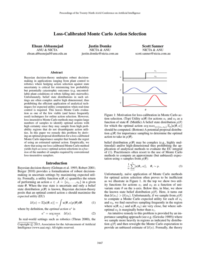
Figure 1: Motivation for loss-calibration in Monte Carlo action selection. (Top) Utility u(θ) for actions a1 and a2 as a
function of state θ. (Middle) A belief state distribution p(θ)
for which the optimal action arg maxa∈{a1 ,a2 } Ep [u(θ, a)]
should be computed. (Bottom) A potential proposal distribution q(θ) for importance sampling to determine the optimal
action to take in p(θ).
belief distribution p(θ) may be complex (e.g., highly multimodal) and/or high-dimensional thus prohibiting the application of analytical methods to evaluate the EU integral
of (1). Practitioners often resort to the use of Monte Carlo
methods to compute an approximate (but unbiased) expectation using n samples from p(θ):
Introduction
n
1X
[u(θ i , a)],
n i=1
Bayesian decision-theory (Gelman et al. 1995; Robert 2001;
Berger 2010) provides a formalization of robust decisionmaking in uncertain settings by maximizing expected utility. Formally, a utility function u(θ, a) quantifies the return
of performing an action a ∈ A = {a1 , . . . , ak } in a given
state θ. When the true state is uncertain and only a belief
state distribution p(θ) is known, Bayesian decision-theory
posits that an optimal control action a should maximize the
expected utility (EU)
ˆ
U(a) = E[u(θ, a)] = u(θ, a)p(θ)dθ.
(1)
where by definition, the optimal action a∗ is
a∗ = arg max U(a).
a
θ i ∼ p.
(3)
Unfortunately, naı̈ve application of Monte Carlo methods
for optimal action selection often proves to be inefficient
as we illustrate in Figure 1. At the top we show two utility functions for actions a1 and a2 as a function of univariate state θ on the x-axis. Below this, in blue, we show
the known state belief distribution p(θ). Here, it turns out
that U(a1 ) > U(a2 ). Unfortunately, if we sample from p(θ)
to compute a Monte Carlo expected utility for each of a1
and a2 , we find ourselves sampling frequently in the region
where u(θ, a1 ) and u(θ, a2 ) are very close, but where suboptimal a2 is marginally better than a1 .
An intuitive remedy to this problem is provided by an importance sampling approach (see e.g. (Geweke 1989)) where
we sample more heavily in regions as indicated by distribution q(θ) and then reweight the Monte Carlo expectation to
provide an unbiased estimate of U(a). Formally, the theory
(2)
In real-world settings such as robotics (Thrun 2000), the
c 2015, Association for the Advancement of Artificial
Copyright Intelligence (www.aaai.org). All rights reserved.
3447
of importance sampling tells us that since
ˆ u(θ, a)p(θ)
U(a) =
q(θ)dθ,
q(θ)
probability and variance operators. We emphasize that all
random variables are determined by q.
In principle, we would like to select the distribution q to
minimize regret, i.e. maximize the true EU of the estimated
action ân . As this is challenging to do directly, we proceed
in three steps:
(4)
we can draw samples from q to compute an (unbiased) estimate of U(a) as
n 1 X u(θ i , a)p(θ i )
, θ i ∼ q.
(5)
Ûn (a) =
n i=1
q(θ i )
1. We establish a connection between regret and the probability of non-optimal action selection in Theorem 1.
2. Since calculating the probability of selecting the nonoptimal action is intractable to be directly minimized, we
derive an upper bound in Theorem 3, based on the variance of the difference of estimated utilities.
This leaves us with one key question to answer in this paper: How can we automatically derive a q(θ) to increase the
probability that the optimal action a∗ is selected for a finite set of n samples? Answering this question is important
for real-time applications of Bayesian decision-theoretic approaches where efficiency and optimality are two key operating criteria.
To this end, in the subsequent section we derive an optimal proposal distribution for a loss-calibrated Monte Carlo
importance sampler. To do this, we first show connections
between regret and the probability of non-optimal action selection and then further connect an upper bound on the latter
to the variance of our expected utility estimator. We are then
able to derive an optimal proposal distribution q that minimizes this variance through the calculus of variations.
We evaluate our loss-calibrated Monte Carlo method
in two domains. We first examine synthetic plant control examples building on those of (Lacoste-Julien, Huszar,
and Ghahramani 2011), who were also motivated by losscalibration in Bayesian decision theory, albeit not in the case
of Monte Carlo methods as we focus on in this work. We also
demonstrate results in a Bayesian decision-theoretic robotics
setting with uncertain localization motivated by the work of
(Thrun 2000).
In both empirical settings and in states with up to 100
dimensions, we demonstrate that using our loss-calibrated
Monte Carlo method yields high-accuracy optimal action
selections in a fraction of the number of samples required by conventional loss-insensitive samplers to achieve
the same level of accuracy. This suggests a new class of
loss-calibrated Monte Carlo samplers for efficient online
Bayesian decision-theoretic action selection.
3. Theorem 5 shows how to calculate the distribution q to
minimize this bound.
Minimizing regret
To find the optimal estimated action ân with fewer samples,
we wish to select q that minimizes the regret. Formally we
define this as
min
q
`(ân )
=
E [U(a∗ ) − U (ân )] .
(7)
Direct minimization of Equation 7 is difficult, hence we
bound it with the probability of selecting a non-optimal action instead. Tightening this bound with respect to q will lead
to a practical strategy. It is detailed in the following theorem.
Theorem 1 (Regret bounds). For the optimal action a∗
and its estimate ân the regret as defined in Equation 7, is
bounded as
∆ P [a∗ 6= ân ] ≤ `(ân ) ≤ Γ P [a∗ 6= ân ] ,
(8)
where ∆ = U(a∗ ) − maxa0 ∈A\{a∗ } U(a0 ) and Γ = U(a∗ ) −
mina0 ∈A U(a0 ).
Proof. We know E [U(ân )] is equal to
X
P [a∗ = ân ] U(a∗ ) +
P [a = ân ] U(a)
a∈A\{a∗ }
∗
∗
≥P [a = ân ] U(a ) +
X
P [a = ân ] min
U(a0 )
0
a ∈A
a∈A\{a∗ }
=P [a∗ = ân ] U(a∗ ) + P [a∗ 6= ân ] min
U(a0 ).
0
Loss-calibrated Monte Carlo Importance
Sampling
a ∈A
This is equivalent to stating that `(ân ) ≤ Γ P [a∗ 6= ân ] after
some manipulation. Similarly, we have that
In many applications of decision theory, sampling is the
most time-consuming step. Since we know these samples
are ultimately used to estimate high-utility actions, we are
interested in guiding the sampler to be more efficient for this
task.
Here, we will pick a distribution q to draw samples from,
which are in turn used to select the action that maximizes
the EU. The estimated optimal action ân from n samples is
defined as
ân = arg max Ûn (a).
(6)
E [U(ân )] ≤ P [a∗ = ân ] U(a∗ ) + P [a∗ 6= ân ]
max
a0 ∈A\{a∗ }
U(a0 )
which leads to `(ân ) ≥ ∆P [a∗ 6= ân ] .
The bound is very intuitive: minimizing the probability
of the estimated optimal action ân being non-optimal will
lead to a bound on the regret. Clearly, for two actions we
have ∆ = Γ. Thus, in the two-action case, minimizing the
probability of selecting a non-optimal action is equivalent to
maximizing the expected utility of the selected action. With
more actions, these objectives are not equivalent, but we can
see that the difference is controlled in terms of ∆ and Γ.
a
Since the samples are drawn randomly from q, ân is a random variable and so is its expected utility U(ân ). As such,
we use E, P and V henceforth to denote the expectation,
3448
Minimizing the probability of non-optimal action
The critical feature of Equation 9 is that all terms on the
RHS other than the variance are constant with respect to the
sampling distribution q. Thus, this theorem suggests that a
reasonable surrogate to minimize the regret in Equation 7
and consequently maximize the expected utility of the estimated optimal action is to minimize the variance of the difference of the estimated utilities. This result is quite intuitive
— if we have a low-variance estimate of the differences of
utilities, we will tend to select the best action.
This is aligned with the importance sampling literature
where it is well known that the optimal distribution to sample from is the one that minimizes the variance (Rubinstein
1981; Glasserman 2004). Our analysis shows the variance
of the function that has to be minimized is of a particular
form that depends on the difference of the utilities (rather
than each utility independently).
∗
We now turn to the problem of minimizing P [a 6= ân ]. In
the following, Lemma 2 provides a bound on the probability
of non-optimal action. Further details and another view of
the same problem with slightly better bounds is provided in
supplementary material.
In the subsequent lemma, we upper bound the indicator
function with a smooth and convex upper bound that will be
easier to minimize. The use of surrogate function for minimizing indicator has also been used in similar problems (see
e.g. (Bartlett, Jordan, and McAaliffe 2006)).
Lemma 2. For an optimal action a∗ and its estimate ân
obtained from sampling, we have ∀t > 0,
P [a∗ 6= ân ] ≤
X X
E
2 t Ûn (a) − Ûn (a0 ) + 1
.
a6=a∗ a0 6=a
Proof. Firstly, decompose P [a∗ 6= ân ] as
X
P[a = ân ] ≤
a6=a∗
X X
a6=a∗
=
Optimal q
We established that to find the optimal proposal distribution
q ∗ (i.e. optimal q), we minimize the sum of variances obtained from Theorem 3. Since a∗ is unknown, we sum over
all actions in A, rather than just A\{a∗ }. Since everything
except variance in Equation 9 is independent of q, we formulate the objective
ˆ
h
i
X X
0
min
V Ûn (a) − Ûn (a ) s.t. q(θ)dθ = 1.
0
P[Ûn (a) > Ûn (a )]
a0 6=a
X X
h h
ii
E I Ûn (a) > Ûn (a0 ) .
a6=a∗ a0 6=a
Applying the inequality that I[v > 0] ≤ (tv + 1)2 gives the result.
q
The next theorem then relates the value inside the above
expectation to the variance, thus bonding the probability of
incorrect action selection by the sum of variances.
Theorem 3 (Upper bound on the probability of non-optimal actions). We have the following upper bound on the
probability of non-optimal action selection for k actions in
set A, true expected utility U(a) and its estimation Ûn (a)
obtained from finite samples:
P [a∗ 6= ân ] ≤
X X
(10)
Here, the constraint on q is to ensure the resulting solution
is a proper probability distribution.
The following theorem provides the solution to the optimization problem in Equation 10 that we are interested in.
Theorem 5. Let A={a1 , . . . , ak } with non-negative utilities. The optimal distribution q ∗ (θ) is the solution to problem in Equation 10 and has the following form:
1 + 2t U(a) − U (a0 )
a6=a∗ a0 6=a
h
a∈A a0 ∈A\{a}
q ∗ (θ) ∝ p(θ)
i
+t2 V Ûn (a) − Ûn (a0 ) +t2 U(a) − U (a0 )
2
!
sX
X
(u(θ, a) − u(θ, a0 ))2 .
(11)
a∈A a0 ∈A\{a}
,
Proof. Since we know V[X] = E[X 2 ] − E[X]2 , for computing the objective in Equation 10 the second expectation
2
becomes (U(a) − U(a0 )) and is independent
of q, then we
(9)
Proof. Expand the quadratic in Lemma 2 and use E[X 2 ] =
V[X] + E[X]2 and E[Ûn (a) − Ûn (a0 )] = U(a) − U(a0 ).
only need to minimize E
Ûn (a) − Ûn (a0 )
2
. Consider this
0
value for a particular pair (a, a ). Denoting Υ(θ i , a, a0 ) =
u(θ, a) − u(θ, a0 ), this is equal to
In general, one would like to select the constant t to minimize this bound. As this depends on the variance, which is a
function of q and the number of samples n, this is difficult to
do analytically. However, we expect the variance to decrease
as n increases, so we instead derive a value for t that leads
to an asymptotically tight upper bound.
Lemma 4. For the bounds detailed in Theorem 3, if the variance term is zero, the value of t that minimizes the upper
bound is
P
P
0
a6=a∗
a0 6=a U(a ) − U(a)
t = P
.
P
0 2
a6=a∗
a0 6=a (U(a) − U(a ))
ˆ
n
q(θ 1,...,n )
1 X Υ(θ i , a, a0 )p(θ i )
n i=1
q(θ i )
!2
dθ 1,...,n
ˆ n n
1 XXΥ(θ i , a, a0 )Υ(θ j , a, a0 )p(θ i )p(θ j )
= 2
n i=1 j=1
q(θ i )q(θ j )
× q(θ 1 , . . . , θ n )dθ 1,...,n .
Since all the samples are independent, q(θ 1 , . . . , θ n ) =
q(θ 1 ) . . . q(θ n ). Now if i 6= j, it is easy to see that q vanishes
and those terms become independent of q. If i = j however,
only one of the terms in the denominator cancels out with the
2
Proof. In general, the value of t minimizing 2ta + t b is
t = −a/b.
3449
joint. Also because the sum is over similar terms, we have n
times the same expression, leading to the Lagrangian of
1 X
n a∈A
ˆ
X
a0 ∈A\{a}
Υ(θ, a, a0 )2 p(θ)2
dθ + λ
q(θ)
ˆ
each action. In case direct sampling is not possible we use
Metropolis-Hastings MCMC by initializing the chain at a
random point and using a Normal distribution centered at the
current sample with isotropic covariance optimally tuned so
that around 23% of samples are accepted (Roberts, Gelman,
and Gilks 1997). In each experiment n samples are generated 200 times and the mean of the percentage of times the
true optimal action is selected is reported.
We include two diagnostics for MCMC samplers: in the
first one (Subsampled MC) we have generated a large chain
of 100000 samples and selected random subsamples to compute the best action using the empirical expected utilities
Ûn (a). Since samples drawn from Markov chains are typically correlated, this diagnosis will help ensure samples are
independent. In the second diagnostic (Sequential MC)
we draw samples sequentially from a single Markov Chain
started at a random point to calculate the expected utilities
for selecting the best action.
q(θ)dθ − 1 .
Taking the derivative with respect to q(θ), we have that
−
1 X
n a∈A
X
a0 ∈A\{a}
Υ(θ, a, a0 )2 p(θ)2
+λ=0
q(θ)2
which concludes the theorem since λn only induces a proportionality constant.
This is quite intuitive – the samples θ will be concentrated
on regions where p(θ) is large, and the difference of utilities
between the actions is large, which is precisely the intuition
that motivated our work in Figure 1. This will tend to lead
to the empirically optimal action being the true one, i.e. that
ân approaches a∗ .
In practice, the normalization constants for p and q are
likely to be unknown, meaning that direct use of Eq. 5 is
impossible. However, there are well-known self-normalized
variants that can be used in practice with p(θ) ∝ p̃(θ) and
q(θ) ∝ q̃(θ), namely
, n
n
1X
p̃(θ i )
1 X p̃(θ i )
Ûn (a) =
u(θ i , a)
θ i ∼ q̃.
n i=1
q̃(θ i )
n i=1 q̃(θ i )
(12)
This simply means that for the case of unnormalized p̃ and
q̃ and letting the n1 terms cancel, the summed utility values
have to now
by the slightly more complex
be.reweighted
Pn p̃(θj ) p̃(θ i )
value of q̃(θi )
j=1 q̃(θ j ) .
Furthermore, as it is hard to directly sample q, we must resort to Markov Chain Monte Carlo (MCMC) methods (Neal
1993), e.g. Metropolis-Hastings (MH). This disregards an
important aspect, namely that the samples we obtain for q
are not truly independent. Rather, the number of effective
samples are affected by the mixing rate of the Markov chain.
Our derivation above does not account for these mixing
rates, which could be important in many applications. For
this reason, our experiments will distinguish between two
settings: First, one can run an extremely long chain, and subsample from this, approximating nearly independent samples as in the derivation above, which we call Subsampled
MC. Second, one can run a single Markov chain, as would be
typical in practice, which we call Sequential MC.
Power-plant Control
We consider a power plant where the temperature of the
generator has to be maintained in a safe range following
the example from (Lacoste-Julien, Huszar, and Ghahramani
2011); the only actions available to achieve this are to turn
the generator on or off. Suboptimal action choices that keep
the generator on in high temperatures or turn it off in unnecessary cases when the temperature is safe and no maintenance is required lead to financial loss for the power plant
and should be avoided.
For this problem, we can model the distribution of the
temperature and use a high utility for cases where a safe action of turning the generator on or off is taken, formally,
(
u(θ, a = on/off) =
Ha
La
(d)
(d)
ca,1 < θ (d) < ca,2
otherwise
(13)
where θ (d) is the d-th dimension of the temperature, Ha , La
(for action a ∈ on/off) is the reward for the given ac(d)
(d)
tion a in the temperature intervals defined by ca,1 and ca,2 .
We use three distinct one dimensional utilities for simu(1)
(1)
(1)
lations: (i) c(1)
on,1 = 15, con,2 = 20, coff,1 = 15, coff,2 =
(1)
21, Hon = 6.5, Hoff = 5, Lon = 1.5, Loff = 4; (ii) con,1 =
(1)
45, con,2
=
(1)
50, coff,1
3, Lon = 1.5, Loff =
(1)
= 35, coff,2
(1)
2.5; (iii) con,1
= 40, Hon = 6.5, Hoff =
(1)
(1)
= 5, con,2 = +∞, coff,1 =
(1)
−∞, coff,2 = +∞, Hon = 5, Hoff = 3, Lon = 2.5, Loff = 3.
Corresponding to each utility, the following three distributions are used to demonstrate how the samples drawn from
p and q ∗ obtained from Theorem 5 perform in selecting the
optimal action:
Applications
As discussed earlier, many applications require optimal actions to be selected efficiently given known (but complex)
p and u. In this section we provide applications and evaluate how well the samples drawn from p and q ∗ compare.
In these simulations we are interested in finding the optimal
action, i.e., the one that maximizes the expected utility, with
the minimum number of samples. As such we generate samples from the true distribution p and the proposed optimal
distribution q ∗ (obtained from Theorem 5 as per the application’s specifications) and compute the expected utilities for
(i) p(θ) = 0.7 ∗ N (θ (1) ; 3, 7) + 0.3 ∗ N (θ (1) ; 12, 2) where
N (θ (1) ; µ, σ 2 ) is a normal distribution with mean µ and variance σ 2 ;
(ii) p(θ) = 0.05 ∗ N (θ (1) ; 3, 1) + 0.2 ∗ N (θ (1) ; 6, 1) + 0.05 ∗
N (θ (1) ; 10, 3) + 0.3 ∗ N (θ (1) ; 15, 2) + 0.05 ∗ N (θ (1) ; 20, 7) +
0.1∗N (θ (1) ; 25, 2)+0.05∗N (θ (1) ; 30, 3)+0.2∗N (θ (1) ; 40, 5)
(iii) a log-normal distribution p(θ) = Log-N (θ (1) ; 0, 1).
3450
distribution of p and q ∗
3
0.02
0.01
2
0
10
θ
20
30
-10
u(θ, on)
u(θ, off)
6
10
θ
20
Probability
4
3
0.025
0.02
0.015
0.01
0.005
20
40
60
0
θ
20
u(θ, on)
u(θ, off)
5
40
0.12
Probability
4
3.5
3
0.08
0.06
0.04
0.02
40
60
θ
60
80
100
20
40
60
θ
80
500
1000
1500
No. Subsamples
80
60
40
20
0
100
500
1000
1500
No. Subsamples
80
60
40
500
1000
1500
No. Subsamples
90
80
70
p
q*
60
0
2000
80
60
40
p
q*
20
0
2000
500
1000
1500
Markov Chain Length
100
2000
100
20
0
100
2000
100
60
0.1
4.5
20
70
θ
% Optimal Action Selected
0
80
0
0.03
5
90
30
0.035
2
Utility Value
0
% Optimal Action Selected
-10
Utility Value
0.03
% Optimal Action Selected
4
0.04
100
% Optimal Action Selected
5
Probability
Utility Value
0.05
Sequential MC
% Optimal Action Selected
u(θ, on)
u(θ, off)
6
Subsampled MC
% Optimal Action Selected
u(θ, a = on/off)
500
1000
1500
Markov Chain Length
2000
100
80
60
40
20
0
p
q*
500
1000
1500
Markov Chain Length
2000
Figure 2: Power-plant simulations: the step-valued utility function (as in Equation 13) in the first column, the true distribution p
(in blue) and q ∗ (in red) in the second column and in the third and forth columns the result of performing Subsampled MC and
Sequential MC (as described in the text) are shown. In the two right-hand columns, note that q ∗ achieves the same percentage
of optimal action selection performance as p in a mere fraction of the number of samples.
ficient. In fact, for a 100-dimensional bimodal Gaussian we
are unable to find the optimal action using only 200 samples
from p, which should be contrasted with the significantly
improved performance given by sampling from q ∗ .
In Figure 2, the utility functions are shown in the first column (with black indicating the utility of on as detailed in
Equation 13) and the temperature distributions (p in blue
as described above and q ∗ in red) in the second column
are shown. In the third and fourth columns the result of
performing Subsampled MC and Sequential MC of the
Metropolis-Hastings sampler for selecting the best action is
shown such that the x-axis represents the number of samples
and the y-axis shows the percentage of times the correct optimal action is selected. Here, in general, we observe that a
significantly smaller number of samples from q ∗ is needed
to select the best action in comparison to the number of samples from p required to achieve the same performance.
To investigate the performance of samples from p and q ∗
in higher dimensions, we use a d-dimensional Gaussian mixture corresponding to temperatures at each point in the plant
as p(θ) = N (θ; 10, Σ) + N (θ; 20, Γ) where 10 and 20 are
d-dimensional vectors with constant value 10 and 20 as the
mean and Σi,j = 5 + I[i = j] and Γi,j = 3 + 7I[i = j] as
d × d covariance matrix. In addition, the utility function in
(d)
(d)
Equation 13 is specified with c(d)
on,1 = 23, con,2 = 25, coff,1 =
% Optimal Action Selected
p
q*
80
60
40
20
0
0
20
40
60
Dimension
80
(a) Subsampled MC
100
% Optimal Action Selected
100
100
p
q*
80
60
40
20
0
0
20
40
60
Dimension
80
100
(b) Sequential MC
Figure 3: Performance of the decision maker in selecting the
best action as the dimension of the problem increases in the
power-plant. Note that at 100 dimensions, p is unable to select the optimal action whereas q still manages to select it
a fraction of the time (and would do better if more samples
were taken).
(d)
20, coff,2 = 22, Hon = 50d, Hoff = 13, Lon = 1.1, Loff =
1.5 log(d). In Figure 3 for d ∈ {2, 4, 10, 20, 50, 80, 100}, we
observe that in an average of 100 runs of the MCMC with
200 samples, as the dimensions increase using q ∗ is more ef-
3451
tion of the robot after taking action a from state θ (that is,
moving from the current location in the direction of the the
selected action heading) and Rr the set induced by region r,
we use the following utility function:


H
u(θ, a) = L

M
% Optimal Action Selected
% Optimal Action Selected
90
80
70
60
0
500
1000
1500
No. Subsamples
(b) Subsampled MC
2000
100
90
80
70
60
0
p
q*
500
1000
1500
Markov Chain Length
(14)
where L < M < H (in our experiments: L = 1, M =
10, H = 400) and a ∈ {forward, backward, right,
left}. Using distribution q ∗ from Theorem 5 as illustrated
in Figure 4a, the samples from q ∗ (in red) concentrated on
the charger’s location which has higher utility value compared to the samples from p (in blue) that are from the mode
of the distribution.
As shown in Figure 4b and 4c, using distribution q ∗ and
running the same diagnostics as the previous experiment we
see significant improvement in selection of the optimal action, requiring only a fraction of the samples of p to achieve
the same optimal action selection percentage.
(a) Environment’s Map
100
(T (θ x , a), T (θ y , a)) ∈ Rcharger
(T (θ x , a), T (θ y , a)) ∈ Rstair ,
otherwise
2000
(c) Sequential MC
Figure 4: A robot’s internal map showing the samples taken
from its true belief distribution p (two modes are shown in
blue, the second one is slightly obfuscated by the robot) and
the optimal sampling distribution q ∗ derived by our loss calibrated Monte Carlo importance sampler in 4a. In 4b and
4c we see the performance (in terms of percentage of optimal action selected) of our loss-calibrated sampling method
using q ∗ leads to near immediate detection of the optimal
action in only a few samples.
Conclusion and Future Work
We investigated the problem of loss-calibrated Monte Carlo
importance sampling methods to improve the efficiency of
optimal Bayesian decision-theoretic action selection in comparison to conventional loss-insensitive Monte Carlo methods. We derived an optimal importance sampling distribution to minimize the regret bounds on the expected utility
for multiple actions. This, to the best of our knowledge, is
the first result linking the utility function for actions and the
optimal distribution for Monte Carlo importance sampling
in Bayesian decision theory. We drew connections from regret to the probability of selecting non-optimal actions and
from there to the variance. We showed using an alternative
distribution as derived in Theorem 5 will sample more heavily from regions of significance as identified by their sum of
utility differences.
Empirically, we showed that our loss-calibrated Monte
Carlo method yields high-accuracy optimal action selections
in a fraction of the number of samples required by lossinsensitive samplers in synthetic examples of up to 100 dimensions and robotics-motivated applications.
Future work should investigate the extension of the novel
results in this work to the case of (a) continuously parameterized actions (Alessandro, Restelli, and Bonarini 2007), (b)
imprecise utility functions (e.g, when the return of a state is
not known precisely, but can be sampled) (Boutilier 2003),
(c) uncontrollable sampling (where the utility partially depends on auxiliary variables that cannot be directly sampled from) and (d) applications in active learning and crowdsourcing (Beygelzimer, Dasgupta, and Langford 2009). Furthermore, the bounds obtained here are not tight in the multiaction setting and can be improved in future work.
Altogether, this work and the many avenues of further
research it enables suggest a new class of state-of-the-art
loss-calibrated Monte Carlo samplers for efficient online
Bayesian decision-theoretic action selection.
Robotics
Another application where sampling has been commonly
used is localization in robotics (Thrun 2000). It is a risksensitive-decision making problem where the robot is rewarded for navigating to the charger in order to maintain its
power but wrong actions may lead to catastrophic incidents
like falling down the stairs or crashing into obstacles. Due
to minimal resources on-board a robot and the nature of the
real-time localization problem, it is crucial for the robot to
be able to select the optimal action rapidly, yet safely.
The state of the robot is the combination of its coordinates on a map and its heading direction. In our example for
these experiments, we use a three dimensional Gaussian belief state distribution with two locations in a room intended
to model that a robot’s belief update has been confused by
symmetries in the environment: one mode is at the robot’s
true location and the other at the opposite end of the room.
In this experiment, we consider a map as shown in Figure
4a where there is a flat in-door environment that the robot
can move by selecting one of the four actions forward, backward, right or left. This action will lead to a movement step
in robot from the current point on map with the heading direction towards the selected action. In doing so however, the
robot has to avoid the stairs (low utility region) and select
the charging source (high utility region).
Assuming a deterministic transition dynamics model
θ 0 = T (θ, a) and denoting (T (θ x , a), T (θ y , a)) as the loca-
3452
Acknowledgements
NICTA is funded by the Australian Government as represented by
the Department of Broadband, Communications and the Digital
Economy and the Australian Research Council through the ICT
Centre of Excellence program.
References
Alessandro, L.; Restelli, M.; and Bonarini, A. 2007. Reinforcement learning in continuous action spaces through sequential monte carlo methods. In Advances in Neural Information Processing Systems.
Bartlett, P.; Jordan, I. M.; and McAaliffe, J. D. 2006. Convexity, classification, and risk bounds. Journal of the American Statistical Association 101(473):138–156.
Berger, J. 2010. Statistical Decision Theory and Bayesian
Analysis. Springer, 2nd edition.
Beygelzimer, A.; Dasgupta, S.; and Langford, J. 2009. Importance weighted active learning. In Proceedings of the
26th Annual International Conference on Machine Learning, ICML ’09, 49–56. New York, NY, USA: ACM.
Boutilier, C. 2003. On the foundations of expected expected
utility. In Proceedings of the 18th International Joint Conference on Artificial Intelligence, IJCAI’03, 285–290. San
Francisco, CA, USA: Morgan Kaufmann Publishers Inc.
Gelman, A.; Robert, C.; Chopin, N.; and Rousseau, J. 1995.
Bayesian Data Analysis. CRC press.
Geweke, J. 1989. Bayesian inference in econometric models
using monte carlo integration. Econometrica 57(6):1317–
1339.
Glasserman, P. 2004. Monte Carlo Methods in Financial Engineering. Applications of Mathematics. Springer, 1st edition.
Lacoste-Julien, S.; Huszar, F.; and Ghahramani, Z. 2011.
Approximate inference for the loss-calibrated bayesian. In
Proceedings of the Fourteenth International Conference
on Artificial Intelligence and Statistics (AISTATS-11), volume 15, 416–424.
Neal, R. M. 1993. Probabilistic inference using markov
chain monte carlo methods. Technical report, University of
Toronto, University of Toronto.
Robert, C. 2001. The Bayesian Choice. Springer Texts in
Statistics. Springer, 2nd edition.
Roberts, G. O.; Gelman, A.; and Gilks, W. R. 1997. Weak
convergence and optimal scaling of random walk metropolis
algorithms. The Annals of Applied Probability 7(1):110–
120.
Rubinstein, R. Y. 1981. Simulation and the Monte Carlo
Method. John Wiley & Sons, Inc., 1st edition.
Thrun, S. 2000. Probabilistic algorithms in robotics. AI
Magazine 21:93–109.
3453