Proceedings of the Twenty-Ninth AAAI Conference on Artificial Intelligence
RANSAC versus CS-RANSAC
Geun-Sik Jo, Kee-Sung Lee, Devy Chandra, Chol-Hee Jang, Myung-Hyun Ga
Department of Computer & Information Engineering
INHA University
Incheon, Korea
gsjo@inha.ac.kr, lee.ks@outlook.kr, wiy_ch4n@hotmail.com, orange@eslab.inha.ac.kr, gagaman7777@eslab.inha.ac.kr
trix generated here depends heavily on the selected random
features. However, RANSAC algorithm picks the features
without considering their locations, which may lead to the
selection of sets of features distributed linearly or too close
to one another, resulting in an inaccurate homography matrix.
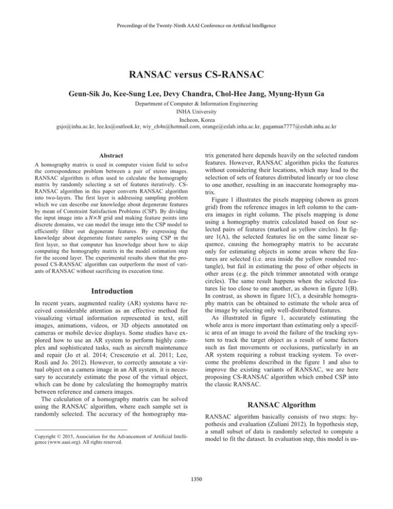
Figure 1 illustrates the pixels mapping (shown as green
grid) from the reference images in left column to the camera images in right column. The pixels mapping is done
using a homography matrix calculated based on four selected pairs of features (marked as yellow circles). In figure 1(A), the selected features lie on the same linear sequence, causing the homography matrix to be accurate
only for estimating objects in some areas where the features are selected (i.e. area inside the yellow rounded rectangle), but fail in estimating the pose of other objects in
other areas (e.g. the pitch trimmer annotated with orange
circles). The same result happens when the selected features lie too close to one another, as shown in figure 1(B).
In contrast, as shown in figure 1(C), a desirable homography matrix can be obtained to estimate the whole area of
the image by selecting only well-distributed features.
As illustrated in figure 1, accurately estimating the
whole area is more important than estimating only a specific area of an image to avoid the failure of the tracking system to track the target object as a result of some factors
such as fast movements or occlusions, particularly in an
AR system requiring a robust tracking system. To overcome the problems described in the figure 1 and also to
improve the existing variants of RANSAC, we are here
proposing CS-RANSAC algorithm which embed CSP into
the classic RANSAC.
Abstract
A homography matrix is used in computer vision field to solve
the correspondence problem between a pair of stereo images.
RANSAC algorithm is often used to calculate the homography
matrix by randomly selecting a set of features iteratively. CSRANSAC algorithm in this paper converts RANSAC algorithm
into two-layers. The first layer is addressing sampling problem
which we can describe our knowledge about degenerate features
by mean of Constraint Satisfaction Problems (CSP). By dividing
the input image into a grid and making feature points into
discrete domains, we can model the image into the CSP model to
efficiently filter out degenerate features. By expressing the
knowledge about degenerate feature samples using CSP in the
first layer, so that computer has knowledge about how to skip
computing the homography matrix in the model estimation step
for the second layer. The experimental results show that the proposed CS-RANSAC algorithm can outperform the most of variants of RANSAC without sacrificing its execution time.
Introduction
In recent years, augmented reality (AR) systems have received considerable attention as an effective method for
visualizing virtual information represented in text, still
images, animations, videos, or 3D objects annotated on
cameras or mobile device displays. Some studies have explored how to use an AR system to perform highly complex and sophisticated tasks, such as aircraft maintenance
and repair (Jo et al. 2014; Crescenzio et al. 2011; Lee,
Rosli and Jo. 2012). However, to correctly annotate a virtual object on a camera image in an AR system, it is necessary to accurately estimate the pose of the virtual object,
which can be done by calculating the homography matrix
between reference and camera images.
The calculation of a homography matrix can be solved
using the RANSAC algorithm, where each sample set is
randomly selected. The accuracy of the homography ma-
RANSAC Algorithm
RANSAC algorithm basically consists of two steps: hypothesis and evaluation (Zuliani 2012). In hypothesis step,
a small subset of data is randomly selected to compute a
model to fit the dataset. In evaluation step, thisPRGHOLVXV
Copyright © 2015, Association for the Advancement of Artificial Intelligence (www.aaai.org). All rights reserved.
1350
determined by the random features and retains only those
whose areas are greater than a given threshold. The threshold value is set to a generous number at the first iteration
and is tightened once the homography matrix becomes
stable. MFF-RS algorithm (Wu and Fang 2007) applies
two filters in the sampling step: angle and length filters.
Each sample feature is considered as a vector and is retained as an inlier only if its value is lower than the median
flow value derived by comparing all the random features.
All these techniques have successfully improved the classic RANSAC algorithm for calculating a data model, particularly the homography matrix of an image pair. However, the resulting homography matrix may not be able to
accurately estimate the pose of objects in the whole image
because they could not express which feature samples are
degenerate samples with the efficient computational model.
Reference image
Camera image
(A) Collinear features set
CSP for RANSAC
Most of artificial intelligence (AI) problems can be formulated as a constraint satisfaction problem (CSP) (Russell,
and Norving 2010) defined by a set of variables
and a set of constraints , where
each variable has a nonempty domain of some possible values . The state of a problem is defined by an assignment of values to some or all of the variables
. An assignment is said to be consistent if it does not violate any constraints, and it is said to
be complete if every variable is mentioned.
A solution to the CSP is then the complete assignment
that satisfies all the constraints (Russell, and Norving
2010). Treating a problem as a CSP confers two important
benefits in vision problems. One is to represent the
knowledge in a form of constraints, the other is to develop
effective and generic heuristics requiring no additional
domain-specific knowledge.
This paper proposes CS-RANSAC algorithm by introducing CSP into a computer vision problem of model estimation, particularly a homography matrix. The sampling
problem of RANSAC algorithm is modeled as a CSP model to help filter out degenerate configurations in this model
(i.e. sets of collinear or adjacent features in the estimation
of a homography matrix), and therefore, gain a homography matrix with higher accuracy to estimate the whole area
of an image.
With the sampling problem of a RANSAC algorithm being considered as a CSP, the variable is defined as a set of
feature points used to calculate the data model, denoted
as with and is the number of samples.
To define the domain and value of each variable, particularly in a model estimation problem for two corresponding
images, the input image is first divided into an grid to allow the CSP model to efficiently check the constraints of each feature pair. The value assignable to each
Reference image
Camera image
(B) Adjacent features set
Reference image
Camera image
(C) Well-distributed features set
Figure 1: Homography matrix calculation by RANSAC
algorithm using different features sets.
ed to determine a consensus set by checking which data
from the dataset are consistent with the model (i.e. the
number of inliers). These steps are iteratively repeated
until the algorithm fails to find a better model to represent
the dataset.
Many studies have been conducted to improve the classic RANSAC algorithm for the calculation of a homography matrix. Some studies focused on finding the true set of
inliers, whereas some others on the sampling step by filtering degenerate samples according to some conditions. LORS algorithm (Chum, Matas, and Kittler 2003) improves
the inlier rate of RANSAC algorithm by locally optimizing
an area of the image that is highly condensed by features.
Here, another RANSAC algorithm is run within each iteration of the RANSAC algorithm. T-RS algorithm (Vincent
and Laganiere 2001) computes the areas of four triangles
1351
Definition 2 (Distance constraints) A set of features satisfies distance constraints iff:
feature is defined as the location of the corresponding cell
where the feature lies in, which can be represented by a
two tuple . Therefore, features lie in the same
cell will be mapped into a same value of a variable. With
this, many degenerate features lying too close to one another can be eliminated. The domain of each feature is a
set of any possible locations of the corresponding cell in
the grid. Together with the constraints defined in next section, this grid helps to reduce the search scope, such
that only one sample can be selected in a cell, and thus,
more time can be spent for some adjacent cells which satisfy constraints.
< > is true
and
< > is true
CS-RANSAC Algorithm
Generally, RANSAC algorithm can be divided into two
main steps: the sampling step and the model estimation
step. CS-RANSAC algorithm modifies the sampling step
of the RANSAC algorithm, where it incorporates a CSP
model to filter out degenerate samples before they can be
used in the model estimation step. As outlined in
Constraints for expressing knowledge about how to
filter out degenerate features
As shown in Table 1, the relationship between all the selected random features is defined using a set of constraints
. In this paper, we employ a set of linear and distance constraints to filter the degenerate samples in a
homography matrix calculation problem to remedy the
problems described in the figure 1. By applying these constraints to Images from UKBench dataset (Nister and
Stewenius 2006), we also would like to verify that CSPbased filtering degenerate features samples generally outperforms other variants of RANSAC algorithm. Linear
constraints ensure that no selected samples lie on the same
linear sequence, whereas distance constraints ensure that
all samples lie far enough from one another.
Algorithm 1 CS-RANSAC.
Input: Extracted features from the input image, the maximum number of sampling iterations , the error
threshold .
1: Initialize = NULL, = 0, =
1, = 0, = 0.
2: Repeat
3:
Initialize = NULL, = NULL, = 0,
= 0, = NULL
4:
While is empty or is not consistent with the
constraints in Definitions 1 and 2 do
5:
If do
6:
Sample features randomly
7:
8:
Check the consistency of according to constraints in Definitions 1 and 2
9:
Else
10:
Sample features based on similarity rankings
11:
+1
12:
Exit While
13:
End If
14:
End While
15:
16:
Calculate based on 17:
Calculate according to 18:
If do
19:
20:
21:
End If
22:
Calculate using Eqn. 1
23:
24: Until Output: Table 1: Features relationships in CS-RANSAC Algorithm
Let be a set of constraints between two features and . is true when both linear and distance constraints are satisfied. With and are the row indices, and and are the column indices of the corresponding cells of features and , respectively, the linear
and distance constraints are defined as follows.
Definition 1 (Linear constraints) A set of features satisfies linear constraints iff:
< > is true and
< > is true and
< > is true
1352
Algorithm 1, features are first selected randomly from
the extracted features of the input image . The sampled
features are then checked for their consistency by the constraints set defined in the previous section. They are considered for the next step only if all the constraints are satisfied. If any pair of features fails to satisfy any constraint,
then CS-RANSAC first checks the sampling iteration denoted as. If exceeds the predefined threshold , then CS-RANSAC instead samples another set of features with the highest similarity ranking
based on the Euclidean distance. Here, is set to 100
sampling iterations to avoid the algorithm to loop forever,
which have not happened or have not even reached to near
that point yet in our real implementation. The rest of the
CS-RANSAC algorithm is similar to that of the classic
RANSAC algorithm, in which the data model is iteratively
calculated and updated using a set of sampled features derived from the previous step (i.e. either the features set
selected by the CSP model or the similarity ranking). The
data model is evaluated based on the number of inliers (i.e.
the number of feature points agrees with the data model
generated in current iteration with respect to an
error threshold ).
The number of iterations of the CS-RANSAC algorithm
is updated at the end of each iteration as follows:
Figure 2: Error rates for various grid sizes and numbers of
features.
Figure 3: Processing times for various grid sizes and numbers of features.
(1)
where is the probability of all sampled features being
inliers, and is set to to obtain high accuracy. Conversely, is the probability of at least one sampled feature
being an outlier, calculated using Eq. 2. Finally, is number of features used to calculate a data model.
Figure 4: Inlier rates for various grid sizes and numbers of
features.
(2)
The data model with the largest number of inliers is retuned as the best data model (i.e. homography matrix )
which corresponds all feature pairs between the source
image and the destination image .
Figure 5: Failure rates for various grid sizes and numbers
of features.
Experiments
image pair are calculated by the Euclidean distance to
generate pairs of matched feature points, which are then
sorted and stored to be used when the proposed CSP model
fails to sample a set of constraints satisfying feature
points. Finally, assuming that all feature points lie in a
real-world plane, the homography matrix for each image
pair is calculated.
Images from UKBench dataset (Nister and Stewenius
2006) with a size of are used for evaluation. A
ground truth tool is built to check the validity of the matching results of the SURF features (Bay et al. 2008) based on
the Euclidean distance. After extracting SURF features
from all test images (i.e. both source and destination
imaJHVWKHVLPLODULW\EHWZHHQH[WUDFWHGIHDWXUHVIURPHDFK
1353
Table 2: Comparison of several variants of RANSAC algorithm for the processing time (ms).
G1
G2
Avg.
Std.
RS
T-RS
79.92
80.96
36.11
38.17
MFF-RS
89.71
38.88
LO-RS
CS-RS
58.34
65.47
27.74
23.12
Avg.
G3
Std.
61.15
67.53
Avg.
G4
Std.
Avg.
G5
Std.
Avg.
33.81
27.17
Std.
35.05
35.75
53.52
51.34
36.38
34.15
67.69
65.60
11.29
10.45
11.54
10.22
66.75
36.44
69.33
36.11
79.77
37.42
11.79
12.96
65.29
52.46
33.80
22.39
44.65
41.43
23.21
21.37
52.13
55.33
17.81
14.74
13.46
9.76
10.33
8.25
Table 3: Comparison of several variants of RANSAC algorithm for the error rate (pixel).
G1
G2
G3
G4
G5
RS
Avg.
81.57
Std.
36.89
Avg.
35.59
Std.
11.62
Avg.
48.01
Std.
22.50
Avg.
128.99
Std.
97.98
Avg.
41.93
Std.
29.80
T-RS
MFF-RS
LO-RS
CS-RS
88.71
99.84
189.74
75.12
104.58
94.69
358.79
26.620
37.28
37.99
217.02
34.51
33.11
14.03
495.21
10.68
48.48
49.00
295.52
44.63
28.56
23.66
845.65
20.48
124.82
157.78
367.95
105.13
76.07
156.88
617.67
46.80
39.12
44.54
227.66
32.30
32.96
43.99
328.79
20.59
Table 4: Comparison of several variants of RANSAC algorithm for the number of inlier.
G1
G2
G3
G4
G5
RS
Avg.
367.04
Std.
Avg.
15.04 2779.16
Std.
Avg.
33.77 1829.35
Std.
24.18
Avg.
272.95
Std.
Avg.
10.00 1637.34
Std.
26.66
T-RS
368.33
14.43 2782.08
32.17 1828.94
22.61
272.19
9.83 1641.83
26.18
MFF-RS
356.22
15.56 2755.89
68.31 1806.23
31.80
261.88
14.11 1625.64
38.21
LO-RS
381.23
14.01 2806.44
14.85 1854.40
13.65
280.45
6.05 1660.93
12.55
CS-RS
371.29
13.10 2788.31
24.12 1837.43
17.00
277.56
6.26 1651.10
18.76
GT
434.58
91.13 2963.75
452.31 1884.14
438.95
306.83
61.83 1709.22
231.93
All matching features are manually verified, one feature
at a time. If there is any pair of features classified as an
inlier (i.e. a pair of corresponding features by the Euclidean distance) but found to be an outlier (i.e. a pair of feature
points that does not match with each other according to
human vision), then it is manually classified as an outlier.
A total of four measures are used to evaluate the proposed
algorithm: error rate, processing time, inlier rate, and failure rate. Error rate refers to the accuracy of the homography matrix, which is derived using the symmetric transfer
error (Hartley and Zisserman 2004) as follows:
Processing time is the time required by each algorithm
to generate a homography matrix for each image pair,
measured on Intel Core I5 CPU 1.80GHz. Inlier rate indicates the probability of features agreeing with .
(4)
Finally, failure rate refers to the rate at which the proposed CSP model fails to find a set of constraints satisfying feature points within 100 sampling iterations.
(3)
where is the Euclidean distance between two feature
points. and are any pixel in the source image and its
estimation in the destination image according to , respectively. A grid is overlaid onto the source image, and is randomly selected from each cell of the grid.
(5)
where is the number of iterations which
use top features by similarity to calculate a homography
matrix, and is the number of iterations required by CS-RANSAC to generate for each image pair.
1354
G1
G2
G3
G4
G5
Figure 6: The classification of test images based on feature distributions (G1: few features distributed over the whole image;
G2: many features distributed over the whole image; G3: many features distributed at the center of the image; G4: few
features distributed over a specific area in the image; G5: many features distributed over a specific area in the image).
times the number of samples, but this comes at the expense
of the processing time when the number of samples is larg
er than four, as shown in figure 3. These results therefore
suggest four as the optimal number of samples and 17×17
as the optimal grid size, as shown in Table 2.
Results and Discussion
Grid Size and Number of Samples for each Image
Though four-point algorithm (Hartley and Zisserman 2004)
has suggested to use sets of four matched points to estimate
a planar homography, this experiment is conducted to determine whether the grid size affects the suggestion of
four-point algorithm. CS-RANSAC algorithm is executed
to calculate a homography matrix for each image pair.
This experiment is conducted on various sizes of grid and
samples using 33 pairs of images, to determine the optimal
grid size and the optimal number of samples for each grid
size in the proposed algorithm. Its performance is evaluated by the error rate, the processing time, the inlier rate, and
the failure rate. The average value of each measure is calculated and presented in graphs, as shown in figures 2, 3,
4, and 5, which clearly show that using four samples indeed is also the optimal number of features in CSRANSAC. Compared to using a larger number of samples,
it produces the lowest error and failure rates, requires the
shortest processing time, and generates the highest inlier
rate.
For the grid size, as shown in figures 2 and 5, the error
and failure rates decrease sharply when the value of N is
three to four times the number of samples. This is because
when the number of samples is greater than or equal to the
value of N, it is not possible to find a set of features that
satisfy all the defined constraints. Therefore, it will invoke
the alternative sampling method and increase the failure
rate. In addition, because the features are selected based
only on their similarity rankings (i.e. there is no guarantee
that the selected samples are well distributed), it increases
the error rate. Similarly, as shown in figure 4, the highest
inlier rate is observed when the value of N is three to four
Table 5: Algorithm behaviors using four features and grid
size of .
Error rate
Processing time
Inlier rate
Failure rate
57.19 pixels
46.38 msec
70.71%
0%
CS-RANSAC vs. Other RANSAC Algorithms
In this experiment, five variants of RANSAC algorithm
with different basic concepts are compared in terms of processing time, error rate, and number of inliers. In CSRANSAC algorithm, as described in previous section, all
the selected samples have to satisfy the defined constraints
to be used in the homography calculation step. In T-RS, the
selected samples are filtered based on the area of triangles
the features form. This only solves the distance problem,
but not the linear problem, which may affect the results.
The constraints in MFF-RS rely only on the length or angle
of the features which are treated as vectors. Therefore,
MFF-RS cannot ensure the distribution of the features. In
contrast, LO-RS focuses only on optimizing the inlier rate,
by employing only the inlier set found in previous steps to
recalculate the homography matrix. With this, the number
of inliers found by LO-RS is expected to be the best among
five variants of RANSAC algorithm in this experiment.
But worth to be noted, the error rate here is calculated
based on the pixel mapping from whole area of the image,
which is why LO-RS has a very high error rate. A total of
50 images are selected and divided into five groups based
on the features distribution pattern (figure 6) such that each
1355
group has 10 pairs of images. Each algorithm is executed
to produce a homography matrix for each image pair. Average (Avg.) and standard deviation (Std.) of the error rate,
the processing time, and the number of inliers are calculated for evaluation.
As shown in Table 3, CS-RANSAC generally provides
better runtime compared to the others, with average reductions ranging from 6% to 20%. This is because only the
constraints satisfying random samples are used, so that it
can produce a correct homography matrix in each iteration
(as shown in Table 4, CS-RANSAC provides lower error
rate compared to other algorithms, with 3% to 85% improvement of the error rate), and thus requires lesser
amount of time to produce the best homography matrix for
each image pair. However, for images in G1 and G4,
which have only a few feature points, LO-RS provides
better execution time than CS-RANSAC by 6% and 12%,
respectively. This is because there are only few features in
the whole image area, so that the proposed CSP model has
difficulty in finding the constraints satisfying features,
which cause the increase of the sampling iteration and
therefore, increase the processing time. For LO-RS, as expected, it provides the largest number of inlier (Table 5,)
and thus it can accurately estimate only specific parts of
the image, reflecting the case shown in figure 1(B).
Because TS-RS does not solve the linear problem, it was
found to have lower accuracy (i.e. higher error rate and
smaller number of inliers) compared to the CS-RANSAC
algorithm. In addition, by dividing the image into a grid, it
helps to eliminate many degenerate features in early steps
without any further calculation. However, T-RS has to
calculate the relationship of each feature before it can eliminate some degenerate ones.
and Stewenius 2006), we proved that the efficient filtering
of degenerate features and guiding how to choose the right
feature samples using CSP can improve overall performance of RANSAC algorithm.
The future work should be improving the CS-RANSAC
algorithm by introducing different constraints for various
types of images, in which the grid size can be also adjusted
and allow CS-RANSAC to automatically select a set of
constraints depending on the distribution pattern of its features.
References
Bay, H.; Ess, A.; Tuytelaars, T.; and Gool, L. V. 2008. SURF:
Speeded Up Robust Features. In Computer Vision and Image
Understanding 110(3): 346-359.
Crescenzio, F. D.; Fantini, M.; Persiani, F.; Stefano, L. D.; Azzari, P.; and Salti, S. 2011. Augmented Reality for Aircraft
Maintenance Training and Operations Support. IEEE Computer
Graphics and Applications 31(1): 96-101.
Hartley, R., and Zisserman, A. 2004. Multiple View Geometry in
Computer Vision Second Edition. Cambridge University Press.
Jo,G.S.; Oh, K.J.; Ha, I.; Lee, K.S.; Hong, M. D.; Neumann, U.;
and You, S. 2014. A Unified Framework for Augmented Reality
and Knowledge-Based Systems in Maintaining Aircraft. In Proceedings of the Twenty-Sixth Annual Conference on Innovative
Applications of Artificial Intelligence/AAAI, 2990-2997.
Lee, K. S.; Rosli, A. N.; and Jo, G. S. 2012. A Method for Automatically Creating an Interactive Semantic Video based on AR
System. In IEEE International Conference on Systems, Man, and
Cybernetics, 2626-2631.
Nister, D., and Stewenius, H. 2006. Scalable Recognition with A
Vocabulary Tree. In IEEE Conference on CVPR 2: 2161-2168.
Russell, S., J., and Norving, P. 2010. Artificial Intelligence: A
Modern Approach Third Edition. Prentice Hall.
Vincent, E., and Laganiere, R. 2001. Detecting Planar Homographies in an Image Pair. In Proceedings of IEEE International
Symposium on Image and Signal Processing and Analysis, 182187.
Conclusions and Future Works
The experimental results show that CS-RANSAC generally
outperforms four other variants of RANSAC algorithm (i.e.
classic RANSAC, T-RS, MFF-RS, and LO-RS) in terms of
accuracy and processing time without sacrificing its execution time. The feature distribution by describing in terms of
CSP strongly affects both the processing time and accuracy
without sacrificing its execution time and inlier rate. Even
though LO-RS provides the highest inlier rate, there is no
significant difference between LO-RS and CS-RS. However, the proposed CS-RANSAC also shows its superiority in
estimating the pose of objects in whole image area, which
can solve the problems described in the figure 1. In addition, it is worth noting that the CSP used in CS-RANSAC
is more general and robust scheme than any other methodology used in four other variants of RANSAC compared in
this research. Through the motivation derived from the
figure 1 and the experiment with UKBench dataset (Nister
Wu, F., and Fang, X. 2004. An Improved RANSAC Homography
Algorithm for Feature Based Image Mosaic. In Proceedings of
WSEAS International Conference on Signal Processing, Computational Geometry & Artificial Vision, 202-207.
Zuliani, M. 2012. RANSAC for Dummies. MathWorks,
URL:http://www.mathworks.com, November 2008.
1356