Proceedings of the Twenty-Eighth AAAI Conference on Artificial Intelligence
Predicting the Hardness of Learning Bayesian Networks
Brandon Malone and Kustaa Kangas and Matti Järvisalo and Mikko Koivisto and Petri Myllymäki
Helsinki Institute for Information Technology & Department of Computer Science, University of Helsinki, Finland
{brandon.malone, juho-kustaa.kangas, matti.jarvisalo, mikko.koivisto, petri.myllymaki}@helsinki.fi
Abstract
Due to the intrinsic differences between the algorithmic approaches underlying the solvers, it is not surprising
that their relative efficiency varies on a per-instance basis.
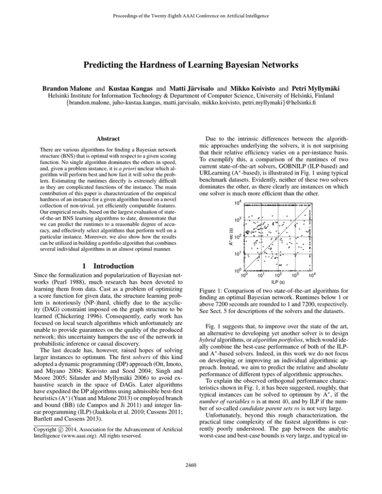
To exemplify this, a comparison of the runtimes of two
current state-of-the-art solvers, GOBNILP (ILP-based) and
URLearning (A∗ -based), is illustrated in Fig. 1 using typical
benchmark datasets. Evidently, neither of these two solvers
dominates the other, as there clearly are instances on which
one solver is much more efficient than the other.
There are various algorithms for finding a Bayesian network
structure (BNS) that is optimal with respect to a given scoring
function. No single algorithm dominates the others in speed,
and, given a problem instance, it is a priori unclear which algorithm will perform best and how fast it will solve the problem. Estimating the runtimes directly is extremely difficult
as they are complicated functions of the instance. The main
contribution of this paper is characterization of the empirical
hardness of an instance for a given algorithm based on a novel
collection of non-trivial, yet efficiently computable features.
Our empirical results, based on the largest evaluation of stateof-the-art BNS learning algorithms to date, demonstrate that
we can predict the runtimes to a reasonable degree of accuracy, and effectively select algorithms that perform well on a
particular instance. Moreover, we also show how the results
can be utilized in building a portfolio algorithm that combines
several individual algorithms in an almost optimal manner.
1
104
A*-ec (s)
103
102
101
Introduction
100 0
10
Since the formalization and popularization of Bayesian networks (Pearl 1988), much research has been devoted to
learning them from data. Cast as a problem of optimizing
a score function for given data, the structure learning problem is notoriously (NP-)hard, chiefly due to the acyclicity (DAG) constraint imposed on the graph structure to be
learned (Chickering 1996). Consequently, early work has
focused on local search algorithms which unfortunately are
unable to provide guarantees on the quality of the produced
network; this uncertainty hampers the use of the network in
probabilistic inference or causal discovery.
The last decade has, however, raised hopes of solving
larger instances to optimum. The first solvers of this kind
adopted a dynamic programming (DP) approach (Ott, Imoto,
and Miyano 2004; Koivisto and Sood 2004; Singh and
Moore 2005; Silander and Myllymäki 2006) to avoid exhaustive search in the space of DAGs. Later algorithms
have expedited the DP algorithms using admissible best-first
heuristics (A∗ ) (Yuan and Malone 2013) or employed branch
and bound (BB) (de Campos and Ji 2011) and integer linear programming (ILP) (Jaakkola et al. 2010; Cussens 2011;
Bartlett and Cussens 2013).
101
102
ILP (s)
103
104
Figure 1: Comparison of two state-of-the-art algorithms for
finding an optimal Bayesian network. Runtimes below 1 or
above 7200 seconds are rounded to 1 and 7200, respectively.
See Sect. 5 for descriptions of the solvers and the datasets.
Fig. 1 suggests that, to improve over the state of the art,
an alternative to developing yet another solver is to design
hybrid algorithms, or algorithm portfolios, which would ideally combine the best-case performance of both of the ILPand A∗ -based solvers. Indeed, in this work we do not focus
on developing or improving an individual algorithmic approach. Instead, we aim to predict the relative and absolute
performance of different types of algorithmic approaches.
To explain the observed orthogonal performance characteristics shown in Fig. 1, it has been suggested, roughly, that
typical instances can be solved to optimum by A∗ , if the
number of variables n is at most 40, and by ILP if the number of so-called candidate parent sets m is not very large.
Unfortunately, beyond this rough characterization, the
practical time complexity of the fastest algorithms is currently poorly understood. The gap between the analytic
worst-case and best-case bounds is very large, and typical in-
c 2014, Association for the Advancement of Artificial
Copyright Intelligence (www.aaai.org). All rights reserved.
2460
and a joint distribution P over the Xi s that factorizes into a
product of the conditional distributions P (Xi |Gi ). Here Gi
is the set of parents of Xi ; a variable Xj is a parent of Xi ,
and Xi a child of Xj , if G contains an arc from Xj to Xi .
Structure learning in Bayesian networks concerns finding
a DAG G that best fits some observed data on the variables.
A good fit can be specified by a real-valued scoring function s(G). Frequently used scoring functions, such as those
based on (penalized) likelihood, MDL, Bayesian principles
(e.g., BDeu and other forms of marginal likelihood), decompose into a sum of local scores si (Gi ) for each variable and
its parents (Heckerman, Geiger, and Chickering 1995). For
each i the local scores are defined for all the 2n−1 possible
parent sets. This number is greatly reduced by enforcing a
small upper bound for the size of the parent sets Gi or by
pruning (de Campos and Ji 2011), as preprocessing, parent
sets that provably cannot belong to an optimal DAG, resulting in a collection of candidate parent sets denoted by Gi .
This motivates the following formulation of the Bayesian
network structure learning problem (BNSL): given local
scores si (Gi ) for a collection of candidate parent sets Gi ∈
Gi , for i =
P1, . . . , n, find a DAG G that minimizes the score
s(G) = i si (Gi ). Along with the number of variables n,
another key parameter describing the size of the input is the
total number of candidate parent sets m = |G1 | + · · · + |Gn |.
stances fall somewhere in between. Moreover, the sophisticated search heuristics employed by the algorithms are quite
sensitive to small variations in the instances, which results
in somewhat chaotic looking behavior of runtimes. Even the
following basic questions are open:
Q1 Are the simple features, the number of variables n and
the number of candidate parent sets m, sufficient for determining which of the available solvers is fastest for a
given instance?
Q2 Are there other efficiently computable features that capture the hardness of the problem significantly more accurately than n and m alone?
In this paper, we answer both these questions in the affirmative. Our results are empirical in that they rely on training and testing a model with a large set of problem instances
collected from various sources. We answer Q1 by learning
a simple, yet nontrivial, model that accurately predicts the
fastest solver for a given instance based on n and m only.
We show how this yields an algorithm portfolio that almost
always runs as fast as the fastest algorithm, thus significantly
outperforming any fixed algorithm on a large collection of
instances. However, a closer inspection reveals that the predicted runtimes often differ from the actual runtimes by one
to two orders of magnitude. To address this issue and answer
Q2, we introduce and study several additional features that
potentially capture the hardness of the problem more accurately for a given solver. We focus on two specific solvers, an
A∗ implementation (Yuan and Malone 2013) and ILP implementation (Bartlett and Cussens 2013), as these turn out to
dominate the other solvers in our empirical study. In particular, we show that learning models with a much wider variety
of features yields significant improvement in the prediction
accuracy: by an order of magnitude for A∗ and close to that
for ILP. Significant in its own right, the empirical work associated with this paper also provides the most elaborate empirical evaluation of state-of-the-art solvers to date.
3
Related Work The idea of learning to predict an algorithm’s runtime from empirical data is not new. Rice (1976)
proposed feature-based modeling to facilitate the selection of the best-performing algorithm for a given problem instance, considering various example problems. Later
works (Carbonell et al. 1991; Fink 1998; Lobjois and
Lemaı̂tre 1998) demonstrated the efficacy of applying machine learning techniques to learn models from empirical
performance data. A Bayesian approach was proposed by
Horvitz et al. (2001). More recently, empirical hardness
models (Leyton-Brown, Nudelman, and Shoham 2002) have
been used in solver portfolios for various NP-hard problems,
such as Boolean satisfiability (SAT) (Xu et al. 2008), constraint programming (Gebruers et al. 2005), and Quantified
Boolean formulas (Pulina and Tacchella 2008). To the best
of our knowledge, for the problem of learning Bayesian networks, the present work is the first to adopt the approach.
2
Capturing Hardness
The hardness of a BNSL instance, relative to a given solver,
is the runtime of the solver on the instance. This extends
to a set of solvers by taking the minimum of the solvers’
runtimes. As long as we consider only deterministic solvers,
the hardness is hereby a well-defined mapping from BNSL
instances to real numbers (extended with ∞), even if presumably computationally hard to evaluate.
We aim to find a model that approximates the hardness
function and is efficient to evaluate for any given instance.
To this end, we work with the hypothesis that an accurate
model can be built based on a small set of efficiently computable features of BNSL instances. We can then learn the
model by computing the feature values and collecting empirical runtime data from a set of BNSL instances. In what follows, we will first introduce several candidate features that
are potentially informative about the hardness of BNSL instances for one or more solvers. A vast majority of these
features have not been previosly considered for characterizing the difficulty of BNSL. We then explain how we learn a
hardness model and estimate its prediction accuracy.
Features for BNSL
We consider several features which naturally fall into four
categories, explained next, based on the strategy used to
compute them: Basic, Basic extended, Lower bounding,
and Probing. Table 1 lists the features in each category.
The Basic features include the number of variables n and
the mean number of candidate parent sets per variable, m/n,
that can be viewed as a natural definition of the “density” of
an instance. The features in Basic extended are other simple features that summarize the size distribution of the collections Gi and the parent sets Gi in each Gi . In the Lower
Learning Bayesian Networks
A Bayesian network (G, P ) consists of a directed acyclic
graph (DAG) G on a set of random variables X1 , . . . , Xn
2461
and output the best DAG found so far. Furthermore, the A∗
and ILP implementations give guaranteed error bounds on
the quality of the found DAGs; an error bound can also be
calculated for the DAG found using greedy hill climbing by
using the lower bounding techniques discussed above. Probing is implemented in practice by running each algorithm for
5 seconds and then collecting several features, including inand out-degree statistics and error bound. We refer to these
feature subcategories of Probing as Greedy probing, A∗
probing, and ILP probing, respectively.
bounding category, the features reflect statistics from a directed graph that is an optimal solution to a relaxation of
the original BNSL problem. In the Simple LB subcategory,
a graph is obtained by letting each variable select its best
parent set according to the scores. Note that the resulting
graph may contain cycles and that the associated score is
a lower bound on the score of an optimal DAG. Many of
the reviewed state-of-the-art solvers use this lower bounding technique; however, they have not used this information
to estimate the difficulty of a given instance. The features
summarize structural properties of the graph: in- and outdegree distribution over the variables, and the number and
size of non-trivial strongly connected components (SCCs).
In the Pattern database LB subcategory, the features are
the same but the graph is obtained by solving a more sophisticated relaxation of the BNSL problem using the pattern
databases technique (Yuan and Malone 2012).
Probing refers to running a solver for several seconds
and collecting statistics about its behavior during the run.
We consider three probing strategies: greedy hill climbing
with a TABU list and random restarts, an anytime variant of
A∗ (Malone and Yuan 2013), and the default version of ILP
(Bartlett and Cussens 2013). All of these algorithms have
anytime characteristics, so they can be stopped at any time
Model Training and Evaluation
Based on the features discussed in the previous section, we
trained models to predict the runtime of an instance of BNSL
for a particular solver. As the models, we considered both
reduced error pruning trees (REP trees) (Quinlan 1987) and
M50 trees (Wang and Witten 1997). Briefly, REP trees are
decision trees which contain a single value in each leaf; that
value is predicted for all instances which reach that leaf. M50
trees are also decision trees; however, each leaf in these trees
contains a linear equation which is used to calculate predictions for instances which reach that leaf. We chose these
decision tree models because of their interpretability, compared to techniques such as neural networks or support vector machines, and because of their flexibility, compared to
linear regression and less expressive model classes.
We evaluated the portfolios using the standard 10-fold
cross-validation technique. That is, the data is partitioned
into 10 non-overlapping subsets. In each fold, 9 of the subsets are used to train the model, and the remaining set is used
for testing; each subset is used as the testing set once. For the
instances in the testing set, we predicted the runtime of each
solver using the model learned with the training set. We then
either selected the solver with the lowest predicted runtime
(and examined its actual runtime against the runtime of the
fastest solver) or compared the predicted runtimes to the actual runtimes. The overall performance of the portfolio is the
union of its performance on each test subset.
Table 1: BNSL features
Basic
1. Number of variables
2. Mean number of CPSs (candidate parent sets)
Basic extended
3–5. Number of CPSs max, sum, sd (standard deviation)
6–8. CPS cardinalities max, mean, sd
Lower bounding
Simple LB
9–11. Node in-degree max, mean, sd
12–14. Node out-degree max, mean, sd
15–17. Node degree max, mean, sd
18. Number of root nodes (no parents)
19. Number of leaf nodes (no children)
20. Number of non-trivial SCCs (strongly connected
components)
21–23. Size of non-trivial SCCs max, mean, sd
Pattern database LB
24–38. The same features as for Simple LB but calculated
on the graph derived from the pattern databases
Probing
Greedy probing
39–41. Node in-degree max, mean, sd
42–44. Node out-degree max, mean, sd
45–47. Node degree max, mean, sd
48. Number of root nodes
49. Number of leave nodes
50. Error bound, derived from the score of the graph and
the pattern database lower bound
A∗ probing
51–62. The same features as for Greedy probing but calculated on the graph learned with A∗ probing
ILP probing
63–74. The same features as for A∗ probing but calculated
on the graph learned with ILP probing
4
Experiment Setup
Solvers
Our focus is on complete BNSL solvers that are capable of producing guaranteed-optimal solutions. Specifically,
we evaluate three complete approaches: Integer-Linear Programming (ILP), A∗ -based state-space search (A∗ ), and
branch-and-bound (BB). The non-default parameterizations
of the solvers were suggested to us by the solver developers.
ILP. We use the GOBNILP solver, version 1.4.1 (http:
//www.cs.york.ac.uk/aig/sw/gobnilp/) as a representative for ILP. GOBNILP uses the SCIP framework
(http://scip.zib.de/) and an external linear program
solver; we used SCIP 3.0.1 and SoPlex 1.7.1 (http://
soplex.zib.de/). In the experiments reported in this paper, we consider two options for GOBNILP. First, in addition to using nested integer programs, it can either search for
BNSL-specific cutting planes using graph-based cycle finding algorithms (ILP) or not (ILP-nc). Second, it can either
2462
5
enforce a total ordering on the variables (-to) or not. In total, we evaluated four parameterizations of the GOBNILP
implementation (ILP, ILP-nc, ILP-to, ILP-nc-to).
A∗ . We use the URLearning solver (http://url.cs.
qc.cuny.edu/software/URLearning.html) as a representative for A∗ . The URLearning implementation of A∗
includes several options which affect its performance on different instances: it can use either a list (A∗ ) or a tree (A∗ tree) for internal computations; it can use either static pattern
databases, dynamic pattern databases (-ed3) or a combination of the two (-ec); pruning behavior is controlled by using
an anytime variant (-atw) or not. In total, we considered six
parameterizations of the URLearning implementation (A∗ ,
A∗ -ed3, A∗ -ec, A∗ -tree, A∗ -atw, A∗ -atw-tree).
BB. We use the sl solver (http://www.ecse.rpi.
edu/˜cvrl/structlearning.html) as a representative
of BB. The sl implementation does not expose any parameters to control its behavior.
Portfolios for BNSL
This section focuses on the construction of practical BNSL
solver portfolios in order to address question Q1. Optimal
portfolio behavior is to always select the best-performing
solver for a given instance. As the main results, we will
show that, perhaps somewhat surprisingly, it is possible to
construct a practical BNSL solver portfolio that is close-tooptimal using only the Basic features.
As the basis of this work, we ran all the solvers and their
parameterizations on all the benchmark instances. Fig. 2
shows the number of instances for which each solver was
the fastest. Here we note that, among the ILP parameterizations, the default version performs the best. For A∗ ,
the A∗ -ec parameterization outperforms the other variants;
more details are available in an online supplement at http:
//bnportfolio.cs.helsinki.fi/. The performance of
BB is in general inferior to the other solvers; in the following we will focus on ILP and A∗ -ec. However, recall
Fig. 1: while ILP is clearly best measured in the number
of instances solved the fastest, the performance of ILP on a
per-instance basis is very much orthogonal to that of A∗ . We
now show that a simple BNSL solver portfolio can capture
the best-case performance of both of these approaches.
Benchmark Datasets
Our training data includes 48 distinct datasets:
• Datasets sampled from benchmark Bayesian networks,
downloaded from http://www.cs.york.ac.uk/aig/
sw/gobnilp/. 19 datasets.
• Datasets originating from the UCI repository (Bache and
Lichman 2013). 19 datasets.
• Datasets sampled from synthetic Bayesian networks. We
generated random networks of varying number of nodes
(20–60) and edges (80-150), and sampled 2000 data
points from each. 7 datasets.
• Datasets we compiled by collecting letter and word occurrences in log files. 3 datasets.
We preprocessed each dataset by removing all continuous variables, variables with very large domains (e.g.
unique identifiers), and variables that take on only one
value. We considered 5 different scoring functions1 : BDeu
with the Equivalent Sample Size parameter selected from
{0.1, 1, 10, 100} and the BIC scores. For each dataset and
scoring function, we generated scores with parent limits
ranging from 2 to up to 6. Due to score pruning, some parent
limits for some datasets result in the same set of local scores;
we removed these duplicates. In total, we obtained 713 distinct instances. The size of the datasets ranged from about
100 records to over 60, 000 records. For portfolio construction we removed very easy instances (solved within 5 seconds by all solvers) as uninteresting, and instances on which
all solvers failed, leaving 586 instances2 .
For running the experiments we used a cluster of Dell
PowerEdge M610 computing nodes equipped with two 2.53GHz Intel Xeon E5540 CPUs and 32-GB RAM. For each
individual run, we used a timeout of 2 hours and a 28-GB
memory limit. We treat the runtime of any instance as 2
hours if a solver exceeds either the time or memory limit.
A Very Simple Solver Portfolio
We found that using only the Basic features (number of variables and mean number of candidate parent sets) are enough
to construct a highly efficient BNSL solver portfolio. We
emphasize that, while on an intuitive level the importance of
these two features may be to some extent unsurprising, such
intuition does not directly translate into an actual predictor
that would close-to-optimally predict the best-performing
solver. Moreover, only two solver parameterizations, ILP
and A∗ -ec are enough for reaching close-to-optimal performance when compared to all the solvers and their parameterizations we considered.
Fig. 3 shows the performance of each individual solver
parameterization, as well as the Virtual Best Solver (VBS),
which is the theoretically optimal portfolio which always selects the best algorithm, constructed by selecting a posteriori the fastest solver for each input instance. “portfolio” is
our simple portfolio which uses only the Basic features and
the ILP and A∗ -ec solvers, constructed and evaluated as described in Sect. 3. REP trees were the base model in this
350
300
250
200
150
100
50
0
1
BB ee
-tr
A* d3
-e
A* c
e
-e re
A* tw-t
-a
A* tw
-a
A*
o
A* c-t
n
PIL o
t
PIL c
-n
P
IL
P
IL
In our experiments, the results were not very sensitive to the
scoring function, except its effect on the number of CPSs, so our
results can generalize to other decomposable scores as well.
2
This is in line with related work on portfolio construction in
other domains such as SAT (Hutter et al. 2014).
Figure 2: VBS contributions of each solver, i.e., the number
of instances for which a solver was fastest.
2463
Table 2: The cumulative runtimes of each solving strategy
on all instances. Instances which failed count as 7200s.
Cumulative runtime (s)
140, 213
212, 237
661, 539
1, 917, 293
4, 149, 928
portfolio (M5’ trees are discussed in Sect. 6). As Table 2
shows, the performance of our simple portfolio is very close
to the theoretically optimal performance of VBS and greatly
outperforms the individual solvers.
For more in-depth understanding, Fig. 4 gives more insight into the effect of the Basic features on the solver runtimes. We observe that the runtimes of A∗ -ec and ILP correlate well with the number of variables (Fig. 4, left) and the
mean number of candidate parent sets (Fig. 4, center).
6
Predicting Runtimes
To address Q2, i.e. the harder task of predicting per-instance
runtimes of individual solvers, and investigate the effect of
the feature sets (cf. Sect. 3) on runtime prediction accuracy.
As just shown, the Basic features can effectively distinguish between solvers to use on a particular instance of
BNSL. However, notable improvements in runtime prediction accuracy are gained by employing a much wider range
of features. In the following we present prediction results for
the REP tree models; see the online supplement for results
using M50 trees. Fig. 5 (left) compares the actual runtimes
for A∗ -ec to the predictions made by the REP tree model
trained using only the Basic features. The model clearly
splits the instances into only a few bins and predicts the
same runtime for all instances in the bin. The actual runtime ranges are quite wide within each bin. For example, for
the bin with predictions near 80 seconds, the actual runtimes
span from around 5 seconds to about an hour. Even though
these predictions allow for good portfolio behavior, they are
not useful to estimate actual runtime.
On the other hand, Fig. 5 (right) shows the same comparison for models learned using A∗ probing features (1–38,
51–62). Many more of the predictions fall along or near the
main diagonal. That is, the larger, more sophisticated feature set results in more accurate runtime predictions. We ob-
500
400
For additional insight, we look at the complexity of the
learned REP trees to predict the runtimes for A∗ -ec and
ILP. As Table 3 shows, for A∗ -ec, given the simple features,
the trees are rather simple, but they become somewhat more
VBS
portfolio
ILP
A*-ec
BB
runtime predicted by basic (s)
number of instances solved
600
REP Tree Characteristics
300
200
100
0
100
10
1
2
10
time (s)
3
10
104
runtime predicted by probing (s)
Algorithm
VBS
portfolio
ILP
A∗ -ec
BB
served similar, though less pronounced, trends for ILP (see
the online supplement for details).
We also evaluated the impact of incrementally adding sets
of features. Fig. 6 shows how the prediction error changes
as we incrementally add Basic (features 1–2), Basic extended (1–23), Lower bounding (1–38), and the relevant
probing features for both A∗ -ec (1–38, 51–62) and ILP (1–
38, 63–74); results for Greedy probing and all features fall
in-between these; see the online suppliment for details. The
figure clearly shows that some features help more than others for the different algorithms. For example, the Basic extended features do not improve the A∗ -ec predictions compared to the Basic features. On the other hand, the extra information about CPSs significantly improves the ILP predictions. The size and difficulty of the linear programs solved
by ILP are directly affected by the CPSs, so the performance of our predictor agrees with our intuition about how
the algorithm behaves. Similarly, the addition of the Lower
bounding features greatly improves the predictions of A∗ ec compared to the Basic and Basic extended features. The
efficacy of the lower bound heuristics directly impacts the
performance of A∗ -ec. Our predictor again effectively exploits features we intuitively expect to characterize runtime
behavior. Probing offers a glimpse at the true runtime behavior of the algorithms, and the predictor leverages this information to further improve prediction accuracy. The results
clearly show that predictions using the Basic features are
much worse than those incorporating the other features. As
in Fig. 5, we see that the more expressive features are necessary for accurate predictions.
Following (Xu et al. 2008), we also trained models which
used multiplicative pairs of features (for all combinations
of feature sets). We observed similar trends regardless of
whether the pairs were included; see the online supplement
for details. We also evaluated the prediction accuracy using
all subsets of features mentioned in Sect. 3. We observed
similar and expected results. For example, ILP probing features did not improve A∗ -ec predictions, and supersets of the
above features yielded similar prediction results.
103
102
101
100 0
10
101
102
103
104
true runtime of A*-ec (s)
104
103
102
101
100 0
10
101
102
103
104
true runtime of A*-ec (s)
Figure 5: Predicted v actual runtimes for A∗ -ec using Basic
features only (left) and all features up to A∗ probing (right).
Figure 3: Solver performance: VBS, our simple portfolio,
ILP, A∗ -ec, and BB.
2464
3
10
2
10
101
100
20
30
40
50
60
70
number of variables
104
runtime of ILP (s)
runtime of A*-ec (s)
104
3
10
2
10
101
100 0
10
1
10
number of variables
2
3
4
5
10
10
10
10
mean number of CPS
6
10
60
50
40
30
20
100
101 102 103 104 105
mean number of CPS
106
Figure 4: Correlation between the Basic features and the runtimes of A∗ -ec (left) and ILP (center). On the right, the two features
plotted against each other and marked depending on whether A∗ is faster (), ILP is faster (), or both solvers fail (×).
Table 3: The size of the REP trees learned for A∗ -ec and ILP.
Algorithm
A∗ -ec
A∗ -ec
ILP
ILP
Features
Basic
A* probing (1–38, 51–62)
Basic
ILP probing (1–38, 63–74)
Depth
3.70 ± 0.48
12.60 ± 1.07
12.60 ± 2.80
11.90 ± 1.20
of features were consistently selected for most of the crossvalidation folds for any particular solver. Qualitatively, this
implies that most of the trees were based on the same small
set of features. Developing a more in-depth understanding of
these instance characteristics in light of solver performance
is an important aspect of future work.
Size (nodes)
11.90 ± 1.20
156.40 ± 17.69
157.20 ± 16.23
206.40 ± 24.68
complex as new features are added. On the other hand, for
ILP, the trees using the additional features do not grow in
depth much. The sizes of the trees show similar behavior3 .
Table 4 shows how often specific features were selected.
A feature is rarely selected for predicting both solvers.
This further confirms that the solver runtimes are influenced
by different structural properties of instances. Nevertheless,
Simple LB features were helpful for both algorithms. Somewhat surprisingly, the Pattern database LB features were
more useful for ILP, even though A∗ -ec directly uses the
pattern database in its search. As shown in Fig. 6, though,
those features do not significantly improve upon the ILP
predictions using Basic extended features. For all of the
graph-based features (node degree and non-trivial SCCs),
the standard deviation was always selected over the maximum and mean. This suggests that systematic variations
between nodes are important for determining the hardness
of an instance. The table also shows that a small number
7
Acknowledgments This work was supported by the
Academy of Finland (grants 251170, 125637, and 255675)
and the Finnish Funding Agency for Technology and Innovation (project D2I). The authors thank James Cussens for
discussions on GOBNILP.
3
The size of the tree can be larger than the number of features
because features can be used at multiple nodes in the tree.
4
absolute prediction error (s)
10
basic
basic extended
w/o probing
probing
103
Table 4: Features used for A∗ -ec and ILP in more than 5
of the 10 cross-validation folds. For each solver, the set of
possible features consisted of non-probing features (1–38)
and the relevant probing features.
102
(1)
(2)
(3)
(4)
(8)
(11)
(14)
(17)
(26)
(38)
(62)
(68)
(74)
1
10
100
200
300 400 500
instance (index)
0
Concluding Remarks
It is possible to construct a surprisingly simple yet highlyefficient BNSL solver portfolio based on a small set of stateof-the-art BNSL solvers, by using machine learning techniques to learn accurate empirical hardness models. Thus the
answer to question Q1 is ‘yes’: a simple model yields a very
efficient algorithm portfolio. Even though the solvers’ runtimes are extremely complicated functions of the instances,
the runtime on a given instance can be relatively accurately
predicted from an extended set of non-trivial but fast-tocompute features. Thus the answer to question Q2 is also
‘yes’: easily computable, more informative features than the
simple m and n are needed in order to improve prediction
accuracy for the solver runtimes. Further improvements to
the predictions are plausible by searching for yet more informative features of BNSL and using other statistical models.
100 200 300 400 500
instance (index)
Figure 6: Prediction errors using different sets of features:
A∗ (left) and ILP (right). Instances are sorted according to
absolute prediction error, defined as the absolute difference
between the actual and predicted runtimes.
2465
Feature
Number of variables, n
Number of CPS, mean
Number of CPS, sum, m
Number of CPS, max
CPS cardinalities, sd
Simple LB, Node in-degree, sd
Simple LB, Node out-degree, sd
Simple LB, Node degree, sd
Pd LB, Node in-degree, sd
Pd LB, Size of non-trivial SCCs, sd
A∗ probing, Error bound
ILP probing, Node out-degree, sd
ILP probing, Error bound
A∗ -ec
10
0
2
0
0
0
8
10
1
0
10
0
0
ILP
0
7
10
7
8
7
0
0
9
8
0
10
10
References
Pearl, J. 1988. Probabilistic reasoning in intelligent systems: networks of plausible inference. Morgan Kaufmann.
Pulina, L., and Tacchella, A. 2008. Treewidth: A useful
marker of empirical hardness in quantified boolean logic encodings. In Proc. LPAR, volume 5330 of LNCS. Springer.
528–542.
Quinlan, J. R. 1987. Simplifying decision trees. International Journal of Man-Machine Studies 27:221–234.
Rice, J. 1976. The algorithm selection problem. Advances
in Computers 15:65–118.
Silander, T., and Myllymäki, P. 2006. A simple approach
for finding the globally optimal Bayesian network structure.
In Proc. UAI, 445–452. AUAI Press.
Singh, A., and Moore, A. 2005. Finding optimal Bayesian
networks by dynamic programming. Technical report,
Carnegie Mellon University.
Wang, Y., and Witten, I. H. 1997. Inducing model trees for
continuous classes. In Proc. ECML Poster Papers, 128–137.
Xu, L.; Hutter, F.; Hoos, H.; and Leyton-Brown, K. 2008.
SATzilla: Portfolio-based algorithm selection for SAT. Journal of Artificial Intelligence Research 32:565–606.
Yuan, C., and Malone, B. 2012. An improved admissible heuristic for finding optimal Bayesian networks. In
Proc. UAI, 924–933. AUAI Press.
Yuan, C., and Malone, B. 2013. Learning optimal Bayesian
networks: A shortest path perspective. Journal of Artificial
Intelligence Research 48:23–65.
Bache, K., and Lichman, M. 2013. UCI machine learning
repository.
Bartlett, M., and Cussens, J. 2013. Advances in Bayesian
network learning using integer programming. In Proc. UAI,
182–191. AUAI Press.
Carbonell, J.; Etzioni, O.; Gil, Y.; Joseph, R.; Knoblock, C.;
Minton, S.; and Veloso, M. 1991. Prodigy: an integrated architecture for planning and learning. SIGART Bulletin 2:51–
55.
Chickering, D. 1996. Learning Bayesian networks is NPcomplete. In Learning from Data: Artificial Intelligence and
Statistics V, 121–130. Springer-Verlag.
Cussens, J. 2011. Bayesian network learning with cutting
planes. In Proc. UAI, 153–160. AUAI Press.
de Campos, C., and Ji, Q. 2011. Efficient learning of
Bayesian networks using constraints. Journal of Machine
Learning Research 12:663–689.
Fink, E. 1998. How to solve it automatically: Selection
among problem-solving methods. In Proc. AIPS, 126–136.
AAAI Press.
Gebruers, C.; Hnich, B.; Bridge, D.; and Freuder, E. 2005.
Using CBR to select solution strategies in constraint programming. In ICCBR, volume 3620 of LNCS, 222–236.
Springer.
Heckerman, D.; Geiger, D.; and Chickering, D. 1995. Learning Bayesian networks: The combination of knowledge and
statistical data. Machine Learning 20:197–243.
Horvitz, E.; Ruan, Y.; Gomes, C. P.; Kautz, H. A.; Selman,
B.; and Chickering, D. M. 2001. A Bayesian approach to
tackling hard computational problems. In Proc. UAI, 235–
244. Morgan Kaufmann.
Hutter, F.; Xu, L.; Hoos, H. H.; and Leyton-Brown, K. 2014.
Algorithm runtime prediction: Methods and evaluation. Artificial Intelligence 206:79 – 111.
Jaakkola, T.; Sontag, D.; Globerson, A.; and Meila, M. 2010.
Learning Bayesian network structure using LP relaxations.
In Proc. AISTATS, 358–365.
Koivisto, M., and Sood, K. 2004. Exact Bayesian structure
discovery in Bayesian networks. Journal of Machine Learning Research 549–573.
Leyton-Brown, K.; Nudelman, E.; and Shoham, Y. 2002.
Learning the empirical hardness of optimization problems:
The case of combinatorial auctions. In Proc. CP, volume
2470 of LNCS, 556–572. Springer.
Lobjois, L., and Lemaı̂tre, M. 1998. Branch and bound algorithm selection by performance prediction. In Proc. AAAI,
353–358. AAAI Press.
Malone, B., and Yuan, C. 2013. Evaluating anytime
algorithms for learning optimal Bayesian networks. In
Proc. UAI. AUAI Press.
Ott, S.; Imoto, S.; and Miyano, S. 2004. Finding optimal
models for small gene networks. In Proc. PSB, 557–567.
World Scientific.
2466