Proceedings of the Twenty-Ninth AAAI Conference on Artificial Intelligence
Pattern-Based Variant-Best-Neighbors Respiratory Motion
Prediction Using Orthogonal Polynomials Approximation
Kin Ming Kam and Shouyi Wang
Stephen R Bowen
Department of Radiology and
Department of Industrial, Manufacturing
& Systems Engineering, University of Texas Integrated Brain Imaging Center,
University of Washington,
at Arlington, TX 76019
Seattle, WA 98195
Wanpracha Chaovalitwongse
Department of Industrial and
Systems Engineering and the Integrated
Brain Imaging Center, University of
Washington, Seattle, WA 98195
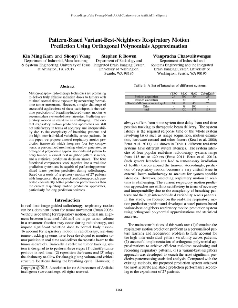
Table 1: A list of latancies of different systems.
Abstract
Motion-adaptive radiotherapy techniques are promising
to deliver truly ablative radiation doses to tumors with
minimal normal tissue exposure by accounting for realtime tumor movement. However, a major challenge of
successful applications of these techniques is the realtime prediction of breathing-induced tumor motion to
accommodate system delivery latencies. Predicting respiratory motion in real-time is challenging. The current respiratory motion prediction approaches are still
not satisfactory in terms of accuracy and interpretability due to the complexity of breathing patterns and
the high inter-individual variability across patients. In
this paper, we propose a novel respiratory motion prediction framework which integrates four key components: a personalized monitoring window generator, an
orthogonal polynomial approximation-based pattern library builder, a variant best neighbor pattern searcher,
and a statistical prediction decision maker. The four
functional components work together into a real-time
prediction system and is capable of performing personalized tumor position prediction during radiotherapy.
Based on a study of respiratory motion of 27 patients
with lung cancer, the proposed prediction approach generated consistently better prediction performances than
the current respiratory motion prediction approaches,
particularly for long prediction horizons.
Position acquisition
Position calculation
Gimbals/MLS/robot control cycle
Other
total
VERO
25
2
20
47
MLC
309
20
52
38
420
MAD
30
45
100
175
CyberKnife
25
15
75
115
always suffers from some system time delay from real-time
position tracking to therapeutic beam delivery. The system
latency is the required response time of the whole system
involving tasks such as image acquisition, motion estimation, hardware control and other factors (Keall et al. 2006;
Ernst et al. 2013). As shown in Table 1, different real-time
systems have different system latencies. The system latencies of four popular real-time radiotherapy systems range
from 115 ms to 420 ms (Ernst 2011; Ernst et al. 2013).
Such system latencies can lead to unnecessary irradiation
of healthy tissues around the tumors. Accordingly, prediction of respiratory motion becomes a very critical issue in
external beam radiotherapy to account for system specific
latencies. However, predicting respiratory motion in realtime is challenging. The current respiratory motion prediction approaches are still not satisfactory in terms of accuracy
and interpretability due to the complexity of breathing patterns and the high inter-individual variability across patients.
In this study, we focused on the real-time respiratory motion prediction problem and developed a novel pattern-based
variant-best-neighbors respiratory motion prediction system
using orthogonal polynomial approximations and statistical
analysis.
Introduction
In real-time image guided radiotherapy, respiratory motion
can be a dominant factor for tumor movement (Ruan 2008).
Without accounting for respiratory motion, critical misalignment between irradiated field and the target tumor volume
in a treatment fraction may occur during radiotherapy, and
impose significant radiation dose to normal body tissues.
To account for respiratory motion in radiotherapy, real-time
tumor-tracking systems have been developed to monitor tumor position in real-time and deliver therapeutic beam to the
tumor accurately. Basically, a real-time tumor tracking system is designed to to perform three steps: (1) identify tumor
position in real time; (2) reposition the beam; and (3) adapt
the dosimetry to allow for changing lung volume and critical
structure locations during the breathing cycle. However, it
The main contributions of this work are: (1) formulate the
respiratory motion prediction problem as a personalized pattern learning and recognition problem to fully account for
the high inter-individual pattern variability across patients.
(2) successful implementation of orthogonal polynomial approximations to achieve efficient real-time monitoring and
recording respiratory patterns, (3) a variant-best-neighbors
approach was developed to search the most significant predictive patterns using statistical analysis. Compared with the
existing methods, the proposed prediction system achieved
the most accurate and stable prediction performance according to the experiment of 27 patients.
c 2015, Association for the Advancement of Artificial
Copyright Intelligence (www.aaai.org). All rights reserved.
1364
Related Work
identified as outliers. Finally, a prediction decision maker
integrates the ‘future values’ of the refined best patterns to
make a prediction.
Many prediction methods for respiratory motion have been
proposed in recent years. In this study, we have studied and reviewed the latest methods including Neural Networks (NN) (Krauss, Nill, and Oelfke 2011), Kernel Density Estimates (KDE) (Ruan 2010), Support Vector Regression Prediction (SVRpred) (Ernst and Schweikard 2009;
Ernst et al. 2013), Recursive Least Squares (RLS) (Ernst et
al. 2013), the MULIN algorithms (Ernst et al. 2013), normalized least mean squares, wavelet-based multiscale autoregression (wLMS) (Renaud, Starck, and Murtagh 2003;
Ernst et al. 2013), Wavelet Neural Network (Chen, Yang,
and Dong 2006), EKF Frequency Tracking. Most recently, Ichiji (Ichiji et al. 2012; 2013a; 2013b) proposed a
Time Varying Seasonal Autoregressive Model with Adaptive Residual (resi-TVSAR) to adapt an AR model to timevarying situation. Ernst et al. (Ernst et al. 2013) did a
comprehensive survey and comparison of the current respiratory motion prediction approaches, and found that the
wLMS approach (Ernst, Schlaefer, and Schweikard 2007;
Renaud, Starck, and Murtagh 2003) achieved the best prediction performance for short term prediction horizons, and
the SVRpred approach (Ernst and Schweikard 2009) using online support vector regression (Renaud, Starck, and
Murtagh 2003) obtained better prediction performance for
longer prediction horizons. It is noted that support vector regression (SVR) is a currently popular approach in
respiratory time series prediction (Choi et al. 2014; Ernst
and Schweikard 2009; Ernst et al. 2013; Guo et al. 2013;
Riaz et al. 2009; Smola and Schölkopf 2004; Bao, Xiong,
and Hu 2014).
Figure 1: The general approach of the proposed patternbased Variant-Best-Neighbors prediction by using raw data.
The Proposed Methods
Most of the current approaches only use recent respiratory
cycles to train a prediction model to account for pattern variations over time. However, the whole respiratory motion
record of a patient is not fully explored and much useful information in the past is not utilized. In this study, we propose
a pattern-matching based framework to identify the similar
patterns from the past respiratory record of a patient, make
predictions based on statistical analysis of the ’future values’ of the identified patterns from past record. Figure 1
shows the system diagram of the proposed prediction framework. Four functional components work together in realtime mode. A sliding window is applied to monitor realtime respiratory motion trajectory, a pattern library builder
performs orthogonal polynomial approximation for the motion pattern within the sliding window, and stores the regression coefficients into the pattern library. The pattern library
is growing over time as the sliding window monitors respiratory motion patterns of the patient. At each step of prediction, a pattern searcher searches a set of best-matching historical patterns in the pattern library to the motion pattern in
the current sliding window. We consider the ‘future values’
of the best-matching historical patterns are useful to predict
the future values beyond the current sliding window. Before
prediction, an outlier analyzer is applied to make statistical
analysis of the future values and eliminates the ones that are
We propose a novel pattern-based variant best neighbors
(VBN) method. For every sliding-window pattern, the number of best-matching neighbors in the pattern library is determined by a pattern-similarity criterion. As shown in Figure 1, before starting prediction, the first step is a training
and validation process to determine the personalized pattern monitoring window length based on the statistics of the
respiratory cycles of each individual patient. As the sliding
window monitors respiratory motion trajectories over time,
a pattern library is built by storing the monitored patterns
in the sliding window. For each step of prediction, the best
matching patterns are selected from the pattern library based
on a pattern-similarity measure. This step provides the most
matching patterns. The next step is to further refine the set
of best neighbors(BNs) to enhance the prediction reliability using statistical analysis. After obtaining the BNs, we
then use ‘future values’ of these patterns to make predictions. One can simply take the average of the ‘future values’
of the BNs or by applying support vector regression. The
performance of both methods will be discussed in result section. Figure 2 illustrates the basic idea of the pattern-based
prediction. Assume three best-matching patterns are identified to be similar to the current sliding window pattern at
time t. For a prediction horizon of h steps, the predicted po-
1365
with k · k being the euclidean norm. Its solution wLS can
be found by setting the derivative with respect to w to zero.
First,
sition at time t + h is a function of the ‘future values’ of the
three best matching neighbors as shown in the Figure.
kFw − yk2 = hFw − y|Fw − yi
= wT FT Fw − 2yT Fw + yT y
(4)
with h·|·i being the standard inner product in a real-valued
vector space. Then,
∂kFw − yk2
= 2FT Fw − 2FT y
∂w
leads to the least-squares solution
(5)
wLS = (FT F)−1 FT y
Figure 2: An example: by using pattern recognition approach, three best neighbors (solid black lines) of the current segment (solid blue line) are identified. By using the
”future” values (the dotted lines) of the best neighbors, the
prediction (red star) is made.
In general, the solution of a linear least-squares problem
is found by conducting a QR decomposition or a singular
value decomposition (SVD) of F. Now, assume that the selected K+1 basis functions are orthogonal with respect to an
PN
inner product yielding the value n=0 fk1 (xn )f˙k2 (xn ) = 0
for any two basis functions fk1 and fk2 with k1 6= k2 . This
is the case for special kinds of polynomials (see Section 3.2),
for wavelet families, or the sinusoidal functions used for discrete Fourier transforms, for instance. Then,
Orthogonal Polynomials Appximation
An orthogonal polynomial sequence is a family of polynomials such that any two different polynomials in the sequence are orthogonal to each other under some inner product (Chihara 2001). Due to convenient mathematical properties, we apply orthogonal polynomials to approximate respiratory motions patterns and do pattern matching correspondingly. The advantages of orthogonal polynomials approximations are: 1. fast determination of best order; 2. signal
smoothing; 3. sparse data representation; 4. accurate approximation; 5. fast update and reconstruction; 6. ready for
clustering and classification by using coefficients.
A time series consisting of real-valued samples yt with
t = 0, ..., N with sampling rate, s, can be modeled by a
parameterized function f (x) : R → R. Here, we assume
that f (x) is linearly dependent on a parameter vector w with
elements wk ∈ R(k = 0, . . . , K). Note that we do not
claim that f (x) is a linear function in x. More concretely,
we assume that f is a linear combination of K + 1 (linear or
nonlinear) so-called basis functions fk :
f (x) =
K
X
wk · fk (x)


f0 (x0 )
···
f0 (xN )
f0 (x0 )


.
.
.


T
..
F F=
.
.
.

.
.
.
.


fK (x0 ) · · · fK (xN )
f0 (xN )


kf0 k2 · · ·
0


. 
 .
..
= .
. 
.
. 
 .
0
· · · kfK k2
..
.
···

fK (x0 )

.

.

.

fK (xN )
(7)
wLS = (FT F)−1 FT y
 

f0 (x0 ) kf10 k2 · · · f0 (xN ) kf10 k2
y
  .0 

..
..
..

=
.
.
.
  .. 

1
1
yN
fK (x0 ) kfK k2 · · · fK (xN ) kfK k2
P

N
yn
f (x )
 n=0 kf0 k2 0 n 


.
..
=

PN

yn
n=0 kfK k2 fK (xn )
(1)
These basis functions may be polynomials, wavelets, sigmoid functions, or sinusoidal functions, for instance. We
may write the values of the K + 1 basis functions for the
N + 1 points in time x0 , . . . , xN into a matrix


f0 (x0 ) · · · fK (x0 )


..
..
F =  ...
(2)

.
.
f0 (xN ) · · · fK (xN )
(8)
That is the least-squares solution can be written as a linear
combination of the training samples (cf. the dual representations of classifiers that are common in the field of support
vector machines, for instance). Assume that, in a time window of length L + 1, the values y0 , y1 , . . . , yL measured at
equidistant points in time x0 , x1 , . . . , xL must be approximated by a polynomial f with degree K ≤ L(L ∈ N0 , K ∈
N0 ) in the least-squares sense.
If we combine the N + 1 samples of the overall time series into a vector y with elements yn , the linear least-squares
problem we want to solve can be denoted by
w
···
That is: FT F is a diagonal matrix which can be inverted
if the elements in the diagonal, which are the squared norms
of the basis functions, are nonzero. This can be easily guaranteed by an appropriate choice of basis functions.
From 6, we then get
k=0
min kFw − yk
(6)
(3)
1366
For sliding window method, the approximation window
[x0 , x1 , . . . , xM ] is located at [0, 1, . . . , L]. Legendre orthogonal polynomials are used in our study. Due to the orthogonality between OPs, the coefficients of OPs are independent to each other. So, if K th order approximation has
been done, we also obtain the approximations of all lower
orders. This property empowers us to efficiently determine
the best order of approximation. For each sliding window
pattern, we first apply a 20th order approximation. To reduce the overfitting issue and smooth out noises, we reconstruct the respiratory motion pattern starting from order 1
until an order such that the approximation R2 > 0.95. The
coefficients of orders higher than this order are set to 0 when
storing into the pattern library.
segments.
SSE
SStot
while the sum of square of errors (SSE) is
2
n
K
n X
X
X
2
|ei | =
∆wk (fk (i) − fk (n))
i=1
i=1 k=1
Sn = 1 −
(11)
(12)
By expansion, the SSE can be written in a close form:
SSE(w) = c11 ∆w12 + c12 ∆w1 ∆w2 + · · · + ckk ∆wk2
(13)
where cjk for j, k ∈ 1, . . . , K which are constants when the
orthogonal polynomials, fk , and n are fixed.
Figure 3 shows the close views of a typical example of
best neighbors found by comparing raw patterns and right
aligned patterns with the current segment. From Figure 3,
we see that right aligned BNs give better prediction result.
Even though the best neighbors found by raw patterns may
show high similarity in overall but the right adjusted best
neighbors show a better matching at the right side which is
the closest point to the point that is going to be predicted.
Personalized Pattern Monitoring Window Size
The interval is measured by the distance between consecutive peaks. The median of it is used as a baseline for window
sizes of two-window design because of the skewness of the
distribution of the interval.
To reasonably determine the final window size, we define
a parameter which is the ratio of window size to the median of the intervals, R, to control the window size. The
R is determined by validation. The window sizes are then
multiplied by the selected ratio, L = Lj × R for j = 1, 2,
i.e. Pattern libraries of all window size Bn×Lj are built up
where n is the number of time segments in the library and
Lj is the size of j th window.
In validation process, one window ratio is picked each
time. R-square is used for performance measurement because it provides a universal metric that describes how close
the prediction is to the real data. The window ratio R that
maximizes the R-square
for prediction.#
" is selected
Pt=n
2
t=1 (ŷ(t, R) − ȳ)
R̂ = arg max 1 − P
(9)
t=n
2
R
t=1 (y(t) − ȳ)
Figure 3: Online prediction of a patient’s respiratory data by
using unaligned BNs(Left) and right-aligned BNs(right).
Then, we sort the list Sn in ascending order to begin acquisition of BNs. We iteratively obtain the BNs from the top
of the list until at least k BNs are obtained, and the next S1
is smaller than the threshold, θ. One important thing has to
be done is to remove the candidates that are adjacent to the
selected BNs in order to prevent bias. Our removal strategy
is shown as below:
Variant Best-Neighbors-Based Predictive Patterns
Phase I: Searching for Initial Best Neighbors By Using
Right Aligned Patterns In phase I-1, the best-matched
patterns are discovered by searching the pattern libraries of
two window sizes, L1 and L2 .
Using the current segment to look for patterns that their
similarity measures, S defined as equation 11, satisfy a similarity threshold, θ. The baseline of candidates must be removed because we are only interested in their patterns. The
regular VBN patterns have the problem of not considering
signal shifting. Thus, it leads to inaccurate prediction due
to the shifted errors as shown in left graphs of Figure 3.
To achieve an accurate prediction, we propose to align the
patterns at their rightmost point during VBN searching process. As shown in Figure 3, the right alignment puts higher
weights on the right end and helps to obtain best neighbors
that have a better match on the right end which is better for
prediction.
ũn = un − un (end)
(10)
Bk = {u ∈ Bk−1 |tu < tλk−1 − m ∪ tu > tλk−1 + m} (14)
where Bk denotes the library at the time of after entering
the kth best neighbor; tλk denotes the time at the end of k th
best neighbor λ; and m denotes a small distance that the
candidates within this range are excluded. In the respiratory
motion prediction study, we choose the distance as one-fifth
of the median of the peak interval, i.e. m = 0.2 × median.
Then, a list of BNs, Bλ , is obtained at the end of Phase I.
Phase II: Best Neighbors Removal By Using Statistical
Analysis Figure 4 shows the scatter plots of the errors
of short segments before and after tλk of the first six best
neighbors of patient 23. This example demonstrates a phenomenon that the error at the right side is positively correlated to the error at the left side. Therefore, by further removing the candidates that have higher errors in the short
where un is the segment of nth candidates in the pattern
library and u0 is the current segment. In this study, we introduce a usage of R-square as a similarity metric of two line
1367
Online Prediction Frameworks Using the Selected
Predictive Patterns
Prediction Using Average of the Future Values of Reference Patterns For the best neighbors, the expected prediction values of h samples ahead is assumed to be similar.
E[y(t + h)] ' E[y(tk + h)] f or k = 1, . . . , K
(18)
where K denotes the number of the similar patterns, y(tk +
h) denotes the value at h samples ahead of kth referenced
pattern. Therefore, the prediction of h samples ahead made
by using k best neighbors can be written as:
Figure 4: Scatter plots of the error before tλ vs the error after
tλ of the first six nearest-neighbors. Correlation between the
errors is observed.
y(t + h) = (t + h) +
Θk · y(tk + h)
(19)
k=1
(t + h) denotes the error of predicting the value at time
t + h and Θk denotes the coefficient of the referenced value
of k th BN. (t + h) includes the random error and pattern
mismatching error.
Taking the average of the referenced values, i.e. the samples that are h samples ahead of all BNs, for prediction, the
proposed model equation can be written as:
term just before tλk , the prediction performance can be enhanced.
The error of the mismatching of a short segment with
length l just before and after time t are significantly correlated, where tc is the current time point of the current segment and tλk is the corresponding time points of k th candidate. To further refine the set of the candidates, we suggest
removing those candidates with bigger mismatching error of
a few points just before time t. The square error of matching
of a short segment of λk is shown as below:
ŷ(t + h) =
K
X
Θ̂k · ŷ(tk + h)
(20)
k=1
dλk = (D(tc − l + 1 : tc ) − D(tλk − l + 1 : tλk ))2 (15)
1
We set Θk = K
to use the mean of the future values of
the referenced patterns for prediction. We name the proposed Right-Aligned Pattern VBN-Based Mean Prediction
as OPPRED and RPKM for the ones using orthogonal polynomials approximation and using raw data respectively.
Next, since the distribution of error are skewed and the
skewness varies among individuals, we remove the candidates with error larger than the median plus one and a half
median absolute deviation(MAD) as follows:
B̃ = {λ ∈ B|dλ <= dmedian + 1.5 × dM AD }
K
X
(16)
Experimental Results
Although it is rare, sometimes the predicted value of a
best-neighbor is an outlier among other candidates as shown
in Figure 5. So, the last step of Phase II is to remove those
candidates as follows:
B̌ = {λ ∈ B|D(tλ + h) < min(max(D(tλ + h)),
(17)
Pλ75 + 1.5 × (Pλ75 − Pλ25 ))}
In our experiments, we compare the prediction performance
of the proposed methods, i.e. RPKM and OPPRED, and
the latest state-of-the-art methods, i.e. wLMS, SVRpred and
TVSAR. In addition, Seasonal ARIMA is also added to the
comparison as most people are familiar to this method.
Data Acquisition and Experimental Settings
Time series of abdominal displacement of 27 lung and liver
cancer patients were collected with the Real-time Position
ManagementTM (RPM)(Varian Inc., Santa Clara, CA) infrared camera and reflective marker block system during
their PET/CT examination. The time series serves as a respiratory motion surrogate (Wang, Gwizdka, and Chaovalitwongse 2014). The sampling rate of respiratory traces
was 30 Hz. The duration of data collection was from 15
to 45 minutes. The respiratory motion traces of 27 patients
demonstrated very high individuality.
For TVSAR and wLMS, they do not need training. Prediction directly started at the testing set. For the experiment of RPKM and OPPRED, the personalized window size
has to be determined before prediction. Also, in the experiment, the similarity threshold θ is set to be 0.95. For SVRpred, we consider −212 , −211 , . . . , 212 for kernel parameter, γ, and 0, 0.01, 0.02, . . . , 0.1 for insensitive zone, , and
max(|ȳ + 3σy |, |ȳ − 3σy ) for regularization parameter, C.
Figure 5: An example of an outlier amongst the best neighbors.
After finalizing the set of BNs, prediction is done by exploiting the information from them. The simplest and effective method is taking an average of their ‘future values’ as
shown in equation 20.
1368
Figure 7: Prediction performance of RPKM, OPPRED,
res TVSAR, wLMS, SVRpred and SARIMA (h=5 steps).
Figure 6: Examples of respiratory motion patterns from six
patients that show the tremendous inter-individual pattern
variability.
Prediction Performance of RPKM, OPPRED and
the latest state-of-the-art methods
Table 2 shows the prediction performances of RPKM, OPPRED, res TVSAR, wLMS, SVRpred and SARIMA. And,
Figure 7 to Figure 9 are the box plots of the prediction performance of the proposed methods and the current stateof-the-art methods for 27 patients. From boxplots, both in
terms of the mean level and the inter-variation of prediction performance of RPKM and OPPRED are significantly
better than all other methods. Among the state-of-the-art
methods, wLMS performs very well in short term prediction and res TVSAR outperforms wLMS for long term prediction. Except SVRpred, all other methods perform better
than SARIMA. From Figure 7 to Figure 9, one can observe
that the RPKM and OPPRED approaches significantly outperform the current methods in all prediction horizons.
Figure 8: Prediction performance of RPKM, OPPRED,
res TVSAR, wLMS, SVRpred and SARIMA (h=10 steps).
Table 2: Prediction performance comparison for the proposed approaches and the state-of-the-art of respiratory motion prediction methods with respect to four prediction hori1
seconds.
zons: 1, 5, 10 and 15 steps. Each step is 30
Prediction horizon (steps)
RPKM
mean
std
OPPRED
mean
std
res TVSAR mean
std
wLMS
mean
std
SVRpred
mean
std
SARIMA
mean
std
1
0.998
0.001
0.998
0.001
0.964
0.088
0.996
0.005
0.908
0.044
0.979
0.019
5
0.976
0.018
0.975
0.019
0.834
0.378
0.880
0.322
0.738
0.075
0.846
0.127
10
0.918
0.052
0.914
0.056
0.684
0.393
0.648
0.487
0.639
0.099
0.608
0.281
15
0.831
0.095
0.824
0.100
0.462
0.436
0.386
0.527
0.347
0.164
0.231
0.469
Figure 9: Prediction performance of RPKM, OPPRED,
res TVSAR, wLMS, SVRpred and SARIMA (h=15 steps).
In real-time radiotherapy, system latencies need to be compensated for accurate irradiation during treatment. Accurate respiratory motion prediction can minimize the damage
of normal body tissues and important human organs. The
proposed approach can effectively utilize the relevant information from the whole respiratory record of a patient. The
orthogonal polynomial approximations have been successfully implemented to achieve efficient real-time monitoring
and recording respiratory patterns. And the variant-bestneighbors approach showed its effectiveness to search the
most significant predictive patterns using statistical analysis.
The experimental results confirmed that the proposed prediction methods outperform all other methods significantly
Discussion and Conclusion
In this study, we developed a pattern-based variant-bestneighbors respiratory motion prediction system using orthogonal polynomial approximations and statistical analysis.
1369
of respiratory motion in radiation oncology report of aapm
task group 76a). Medical physics 33(10):3874–3900.
Krauss, A.; Nill, S.; and Oelfke, U. 2011. The comparative performance of four respiratory motion predictors for
real-time tumour tracking. Physics in medicine and biology
56(16):5303.
Renaud, O.; Starck, J.-L.; and Murtagh, F. 2003. Prediction
based on a multiscale decomposition. International Journal of Wavelets, Multiresolution and Information Processing
1(02):217–232.
Riaz, N.; Shanker, P.; Wiersma, R.; Gudmundsson, O.; Mao,
W.; Widrow, B.; and Xing, L. 2009. Predicting respiratory tumor motion with multi-dimensional adaptive filters
and support vector regression. Physics in medicine and biology 54(19):5735.
Ruan, D. 2008. Image guided respiratory motion analysis:
time series and image registration. ProQuest.
Ruan, D. 2010. Kernel density estimation-based real-time
prediction for respiratory motion. Physics in medicine and
biology 55(5):1311.
Smola, A. J., and Schölkopf, B. 2004. A tutorial on support
vector regression. Statistics and computing 14(3):199–222.
Wang, S.; Gwizdka, J.; and Chaovalitwongse, W. A. 2014.
Using physiological signals to assess mental motion for tumor following radiotherapy. IEEE TRANSACTIONS ON
HUMAN-MACHINE SYSTEMS.
which gives a great impact on respiratory motion time series
prediction for radiotherapy.
References
Bao, Y.; Xiong, T.; and Hu, Z. 2014. Multi-step-ahead
time series prediction using multiple-output support vector
regression. Neurocomputing 129:482–493.
Chen, Y.; Yang, B.; and Dong, J. 2006. Time-series prediction using a local linear wavelet neural network. Neurocomputing 69(4):449–465.
Chihara, T. 2001. 45 years of orthogonal polynomials: a
view from the wings. Journal of computational and applied
mathematics 133(1):13–21.
Choi, S.; Chang, Y.; Kim, N.; Park, S. H.; Song, S. Y.; and
Kang, H. S. 2014. Performance enhancement of respiratory
tumor motion prediction using adaptive support vector regression: Comparison with adaptive neural network method.
International Journal of Imaging Systems and Technology
24(1):8–15.
Ernst, F., and Schweikard, A. 2009. Forecasting respiratory
motion with accurate online support vector regression (svrpred). International journal of computer assisted radiology
and surgery 4(5):439–447.
Ernst, F.; Dürichen, R.; Schlaefer, A.; and Schweikard, A.
2013. Evaluating and comparing algorithms for respiratory motion prediction. Physics in medicine and biology
58(11):3911.
Ernst, F.; Schlaefer, A.; and Schweikard, A. 2007. Prediction of respiratory motion with wavelet-based multiscale
autoregression. Medical Image Computing and ComputerAssisted InterventionMICCAI 2007 668–675.
Ernst, F. 2011. Compensating for quasi-periodic Motion in
robotic radiosurgery. Springer.
Guo, S.; Lucas, R. M.; Ponsonby, A.-L.; et al. 2013. A
novel approach for prediction of vitamin d status using support vector regression. PloS one 8(11):e79970.
Ichiji, K.; Homma, N.; Sakai, M.; Takai, Y.; Narita, Y.;
Abe, M.; and Yoshizawa, M. 2012. Respiratory motion
prediction for tumor following radiotherapy by using timevariant seasonal autoregressive techniques. Engineering in
Medicine and Biology Society (EMBC), 2012 Annual International Conference of the IEEE 8:6028–6031.
Ichiji, K.; Homma, N.; Sakai, M.; Abe, M.; Sugita, N.;
and Yoshizawa, M. 2013a. A respiratory motion prediction based on time-variant seasonal autoregressive model for
real-time image-guided radiotherapy.
Ichiji, K.; Homma, N.; Sakai, M.; Narita, Y.; Takai, Y.;
Zhang, X.; Abe, M.; Sugita, N.; and Yoshizawa, M. 2013b.
A time-varying seasonal autoregressive model-based prediction of respiratory motion for tumor following radiotherapy. Computational and mathematical methods in medicine
2013.
Keall, P. J.; Mageras, G. S.; Balter, J. M.; Emery, R. S.;
Forster, K. M.; Jiang, S. B.; Kapatoes, J. M.; Low, D. A.;
Murphy, M. J.; Murray, B. R.; et al. 2006. The management
1370