Proceedings of the Twenty-Eighth AAAI Conference on Artificial Intelligence
ReLISH: Reliable Label Inference via Smoothness Hypothesis
Chen Gong†,? and Dacheng Tao? and Keren Fu† and Jie Yang†
?
†
Institute of Image Processing and Pattern Recognition, Shanghai Jiao Tong University
Centre for Quantum Computation and Intelligent Systems, University of Technology Sydney
{goodgongchen, fkrsuper, jieyang}@sjtu.edu.cn
dacheng.tao@uts.edu.au
Abstract
Bridge
point
d
The smoothness hypothesis is critical for graph-based
semi-supervised learning. This paper defines local
smoothness, based on which a new algorithm, Reliable
Label Inference via Smoothness Hypothesis (ReLISH),
is proposed. ReLISH has produced smoother labels
than some existing methods for both labeled and
unlabeled examples. Theoretical analyses demonstrate
good stability and generalizability of ReLISH. Using
real-world datasets, our empirical analyses reveal
that ReLISH is promising for both transductive and
inductive tasks, when compared with representative
algorithms, including Harmonic Functions, Local
and Global Consistency, Constraint Metric Learning,
Linear Neighborhood Propagation, and Manifold
Regularization.
+0.0041
+9.006×10-4
d
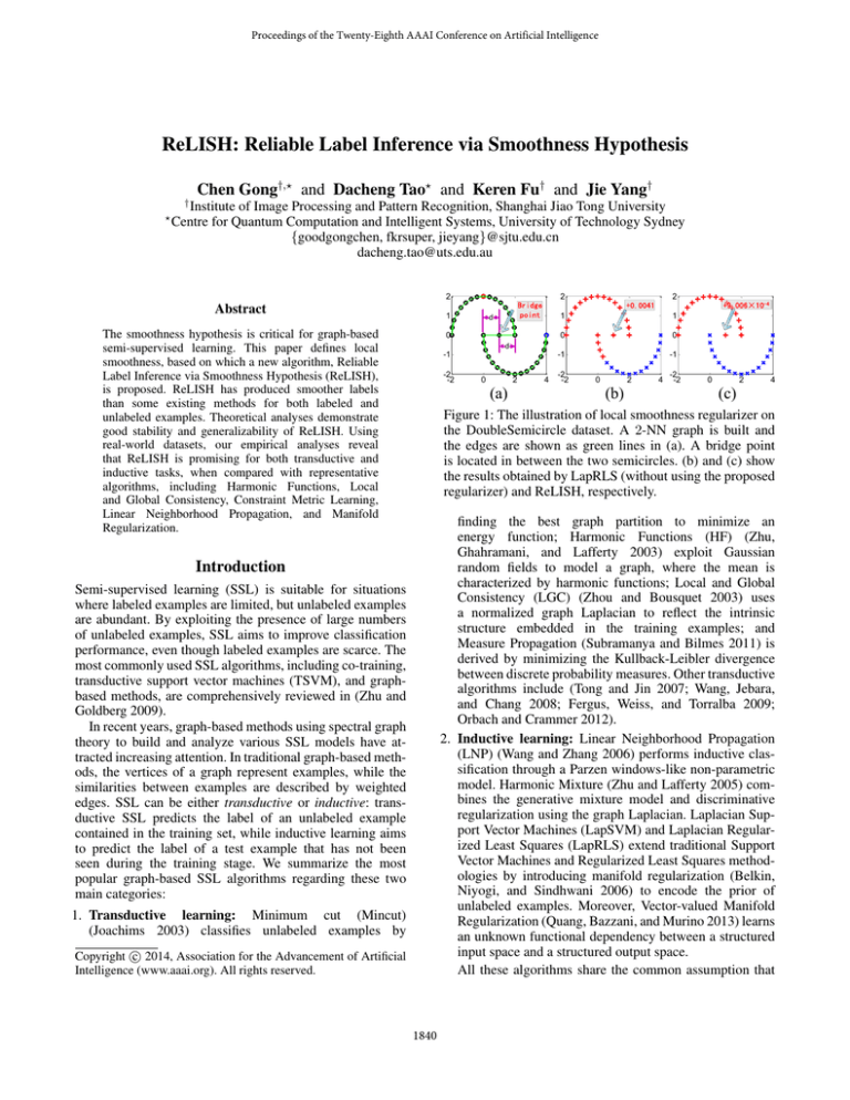
Figure 1: The illustration of local smoothness regularizer on
the DoubleSemicircle dataset. A 2-NN graph is built and
the edges are shown as green lines in (a). A bridge point
is located in between the two semicircles. (b) and (c) show
the results obtained by LapRLS (without using the proposed
regularizer) and ReLISH, respectively.
finding the best graph partition to minimize an
energy function; Harmonic Functions (HF) (Zhu,
Ghahramani, and Lafferty 2003) exploit Gaussian
random fields to model a graph, where the mean is
characterized by harmonic functions; Local and Global
Consistency (LGC) (Zhou and Bousquet 2003) uses
a normalized graph Laplacian to reflect the intrinsic
structure embedded in the training examples; and
Measure Propagation (Subramanya and Bilmes 2011) is
derived by minimizing the Kullback-Leibler divergence
between discrete probability measures. Other transductive
algorithms include (Tong and Jin 2007; Wang, Jebara,
and Chang 2008; Fergus, Weiss, and Torralba 2009;
Orbach and Crammer 2012).
2. Inductive learning: Linear Neighborhood Propagation
(LNP) (Wang and Zhang 2006) performs inductive classification through a Parzen windows-like non-parametric
model. Harmonic Mixture (Zhu and Lafferty 2005) combines the generative mixture model and discriminative
regularization using the graph Laplacian. Laplacian Support Vector Machines (LapSVM) and Laplacian Regularized Least Squares (LapRLS) extend traditional Support
Vector Machines and Regularized Least Squares methodologies by introducing manifold regularization (Belkin,
Niyogi, and Sindhwani 2006) to encode the prior of
unlabeled examples. Moreover, Vector-valued Manifold
Regularization (Quang, Bazzani, and Murino 2013) learns
an unknown functional dependency between a structured
input space and a structured output space.
All these algorithms share the common assumption that
Introduction
Semi-supervised learning (SSL) is suitable for situations
where labeled examples are limited, but unlabeled examples
are abundant. By exploiting the presence of large numbers
of unlabeled examples, SSL aims to improve classification
performance, even though labeled examples are scarce. The
most commonly used SSL algorithms, including co-training,
transductive support vector machines (TSVM), and graphbased methods, are comprehensively reviewed in (Zhu and
Goldberg 2009).
In recent years, graph-based methods using spectral graph
theory to build and analyze various SSL models have attracted increasing attention. In traditional graph-based methods, the vertices of a graph represent examples, while the
similarities between examples are described by weighted
edges. SSL can be either transductive or inductive: transductive SSL predicts the label of an unlabeled example
contained in the training set, while inductive learning aims
to predict the label of a test example that has not been
seen during the training stage. We summarize the most
popular graph-based SSL algorithms regarding these two
main categories:
1. Transductive learning: Minimum cut (Mincut)
(Joachims 2003) classifies unlabeled examples by
Copyright c 2014, Association for the Advancement of Artificial
Intelligence (www.aaai.org). All rights reserved.
1840
l ⌧ u, where xi (1  i  n, n = l +u) are d-dimensional
examples sampled from an unknown marginal distribution
PX , and yi (1  i  l) are labels taking values from a binary
label set {1, 1}. An inductive SSL algorithm aims to find
a suitable hypothesis f : Rd ! R based on the union of L
and U , i.e.
= {(x1 , y1 ), · · · , (xl , yl ), xl+1 · · · xl+u }, to
perfectly predict the label of a test example.
To learn the prediction function f , all examples in are
represented by nodes in a graph G with the adjacency matrix
W, and the similarity between two nodes xi and xj (1 
i, j  n) are defined by an⇣edge in which the weight
is a
⌘
2
2
Gaussian kernel Wij = exp
kxi xj k /(2 ) with the
width . The traditional regularization framework for graphbased SSL is formulated as
1
min E(f ) = [c̃(f (·), x1⇠l , y1⇠l ) + ↵S(f (·), x1⇠n , W)
f
2
+ Q(kf k)] ,
(1)
where the first term is a fidelity function defined on L, which
requests f to fit the labels of the labeled examples; the
second smoothness term enforces labels on the graph that
vary smoothly to reflect the intrinsic geometry of PX ; and
the third induction term controls the complexity of f . Two
free parameters, ↵ and , balance the weights of these three
terms.
The fundamental smoothness assumption widely adopted
in classical graph-based SSL is that if x1 , x2 2 X are close in
the intrinsic geometry of the marginal distribution PX , then
the conditional distributions P (y1 |x1 ) and P (y2 |x2 ) are
similar. A smoother function f on the training set usually
leads to better classification performance for test examples.
Therefore, the smoothness term S(f (·), x1⇠n , W) plays an
important role in the whole regularization framework. In our
method the smoothness term S(f (·), x1⇠n ,W) is defined
by
the learned functions are smooth on the graph, and that a pair
of examples connected by a strong edge are likely to have
similar labels. In this paper we propose a novel regularizer
that introduces local smoothness to describe the relationship
between examples and their neighbors. An example strongly
associated with its neighbors should result in a similar
label in order to achieve sufficient label smoothness in a
local area. Conversely, an example weakly connected to its
neighbors (e.g. an outlier) should not obtain a confident
label. Based on this principle, we propose the Reliable
Label Inference via Smoothness Hypothesis (ReLISH) algorithm, which is theoretically and empirically demonstrated
to improve SSL performance for classification purposes. In
Figure 1, we use the DoubleSemicircle dataset to intuitively
show the effectiveness of proposed local smoothness regularizer. The red, blue and black circles in (a) represent
positive, negative, and unlabeled examples, respectively.
Examples belonging to the top semicircle form the positive
class and examples in the bottom semicircle correspond to
the negative class. The point at (1, 0) lies exactly in the middle of the two classes, and can be attributed to an arbitrary
class. We call this point “bridge point” because it locates in
the intersection area of classes and will probably serve as
a bridge for the undesirable mutual transmission of positive
and negative labels. The simulation in Figure 1 (b) is simply
based on LapRLS which does not incorporate the local
smoothness regularizer, so the positive label is erroneously
propagated to the negative class through the “bridge point”.
By contrast, Figure 1 (c) shows that the proposed ReLISH
equipped with the local smoothness regularizer assigns a
very weak label to the “bridge point”, and successfully
prohibits the label information from passing through it.
Therefore, ReLISH achieves a perfect classification result.
ReLISH is cast into a convex optimization problem and
explores the geometry of the data distribution by postulating
that its support has the geometric structure of a Riemannian
manifold. Our theoretical analyses reveal that the hypothesis determined by ReLISH is very stable, and that the
probability of the generalization risk being larger than any
positive constant is bounded. The proposed algorithm therefore performs accurately and reliably. Moreover, the kernel
extension of ReLISH has been proved to be equivalent to
conducting ReLISH on the data pre-processed by kernel
principal component analysis (KPCA). This profound property indicates all theoretical results of ReLISH are tenable to
its kernel extension.
We conduct comprehensive experiments to compare ReLISH with representative SSL algorithms on several public
datasets, including UCI (Frank and Asuncion 2010), the
Optical Recognition of Handwritten Digits Dataset (Frank
and Asuncion 2010), and Caltech 256 (Griffin, Holub, and
Perona 2007). These empirical studies complement our theoretical studies and show that ReLISH achieves promising
performance on both the transductive and inductive settings.
S(f (·), x1⇠n , W) =
1 Xn Xn
Wij (f (xi ) f (xj ))2
g0
i=1
j=1
2
Xn
+ g1
f 2 (xi )/dii
i=1
= g0 f T Lf + g1 f T D
1
f
(2)
T
where f = (f (x1 ), f (x2 ), · · · , f (xn )) , with f (xi ) 2 R
(1  i  n) representing
Pnthe soft labels obtained by xi . The
degree of xi is dii = j=1 Wij , and the degrees of all the
examples form a diagonal matrix D = diag(d11 , · · · , dnn ).
L = D W is the graph Laplacian, which approximates
the Laplace-Beltrami operator M on a compact manifold
M ⇢ Rd under certain conditions (Belkin and Niyogi 2003).
The first pairwise smoothness term in (2) is defined using
pairs of examples and indicates that two examples sharing
a large edge weight Wij should have similar soft labels.
The second term is the local smoothness term, which is
defined by the connection between xi and its neighbors. This
term considers smoothness of examples in a local region
as a whole, which regularizes the label of xi heavily if it
corresponds to a low degree dii . In Figure 1 (c), the “bridge
point” has lower degree than other points, so its label is regularized to a very small number. From another perspective
Model Description
l
Given a set of labeled examples L = {(xi , yi )}i=1 and a
l+u
set of unlabeled examples U = {(xi )}i=l+1 , typically with
1841
to 0 to explicitly assess the smoothness of ReLISH on
the training set, so⇣ the objective function is simplified ⌘
as
2
1
T
T
1
min E(f1 ) = 2 kJf 1 yk2 + ↵f1 Lf1 + f1 D f1 ,
where the probability distribution PX is supported by a lowdimensional manifold M, then (2) is able to discover the
intrinsic geometry of PX by penalizing f along M.
The regularization framework of ReLISH is derived in the
Euclidian space. Suppose the prediction function is
of which the minimizer is f1 = J+↵L+ D 1
Similarly, the solution of LapRLS is f2 = (J+↵L)
Then the difference between f1T Lf1 and f2T Lf2 is
(3)
f (x) = ! T x,
T
in which !
=
(!1 , · · · , !d )
is a coefficient
vector and x is a test example drawn from PX .
If we put all the training examples in a matrix
X = (x1 , · · · , xl , xl+1 , · · · , xl+u ) = (Xl Xu ) where
each column represents a d-dimensional label vector, then
the induction and fidelity terms in (1) can be defined by
2
2
Q(kf k) = k!k2 and c̃(f (·), x1⇠l , y1⇠l ) = y JXT ! 2 ,
respectively. Here J = diag(1, · · · , 1, 0, · · · 0) is an n ⇥ n
diagonal matrix with the first l elements 1, and the rest are
0. Therefore, the regularization framework of ReLISH is
1h
2
y JXT ! 2 +↵! T XLXT !
min E(!) =
!
2
(4)
i
2
+ ! T XD 1 XT ! + k!k2 ,
f2T Lf2
1
T
T
T
L(J + ↵L)
y.
y.
1
)
1
1
L(J + ↵L + D
1
)
= yT ⌦y.
1
i
y
(7)
According to Lemma 1, ⌦ is a positive semi-definite matrix,
so we have yT ⌦y 0 , which reveals that f1T Lf1  f2T Lf2 .
This completes the proof.
One may argue that a smoother solution can be acquired
by simply increasing the ↵ in (4). However, this way will
significantly weaken the influences of other terms on the
result, which is unfavorable to obtaining satisfactory performances. In this view, ReLISH aims to obtain a smoother
solution as well as not decrease the impacts of other regularizers on the outputs.
Stability and Generalization
This section studies the generalization bound of ReLISH
theoretically, based on the notion of stability proposed by
Bousquet et al. (2001).
XT ! + XJXT !
1
1
(J + ↵L + D
XJy = 0.
(5)
Therefore, by considering Jy = y, the minimizer of (4) is
⇤
1
f1T Lf1
= yT (J + ↵L)
where ↵, , and are non-negative parameters balancing
the weights of these four terms. Note that (4) differs from
LapRLS (Belkin, Niyogi, and Sindhwani 2006) simply in
the local smoothness term ! T XD 1 XT !. The effectiveness of this new regularizer for boosting the classification
accuracy will be theoretically justified in the next section.
To find the optimal ! ⇤ , we set the derivative of the right
hand side of (4) w.r.t. ! to 0, and obtain
! + ↵XLXT ! + XD
h
1
Stability
Definition 3 (Bousquet and Elisseeff 2001): Let
=
{x1 , · · · , xn } be a training set, h = \xh be the training
set where the example xh has been removed, and A is
a symmetric algorithm. We say that A is ✓-stable if the
following inequality holds:
1
Xy. (6)
! = I+↵XLX + XD X +XJX
Finally, the optimal f ⇤ is obtained by plugging (6) into (3).
(8)
8xh 2 , |c(f , x) c(f h , x)|  ✓,
where c(·, ·) is the cost function.
According to Definition 3, we have the following theorem:
=
Theorem
4:
Given
c(f (·), x1⇠l , y1⇠l )
2
1
1
T
c̃(f
(·),
x
,
y
)
=
!
as
the
loss
y
JX
1⇠l 1⇠l
2
2⌘
⇣ 2q
1
8ndl
ndl2
function, ReLISH is 2 1 + l
-stable on the
+ 2
Proof of Smoothness
As mentioned above, graph-based SSL algorithms prefer a
smoother f (Zhu and Goldberg 2009), because it usually
results in higher accuracy. This section proves that the new
local smoothness term makes the label vector f obtained by
ReLISH smoother than that obtained by LapRLS.
Lemma 1: Let D and L be the degree matrix and
graph Laplacian, respectively. J is an n ⇥ n diagonal
matrix of which the first l elements are 1 and the
1
1
rest are 0. Then ⌦ = (J + ↵L) L(J + ↵L)
1
1
1
1
is a positive
(J + ↵L + D ) L(J + ↵L + D )
semi-definite matrix.
Proof is provided in the supplementary material.
Theorem 2: ReLISH is guaranteed to obtain a smoother f
than LapRLS due to the incorporated local smoothness term.
Proof : The smoothness of f is evaluated by
= f T Lf
(Zhu, Ghahramani, and Lafferty 2003; Zhu and Goldberg
2009). Therefore, if f1 and f2 are used to denote the solutions of ReLISH and LapRLS, respectively, then we need
is set
to prove f1T Lf1 is smaller than f2T Lf2 . In (4),
training set = {x1 , · · · , xn }.
Proof is provided in the supplementary material.
Generalization Bound
Pn
2
The empirical risk Rn (f ) = n1 i=1 (f (xi ) yi ) is an
evaluation of how well the hypothesis f fits the training set . The generalization risk expressed by R(f ) =
2
E(f (xi ) yi ) is the expectation of the square loss of f on
the whole example space ⇥ with all xi (1  i  n) sampled
from ⇥.
Theorem 5 (Bousquet and Elisseeff 2001): Let A be a ✓stable algorithm, so that 0  c(f (·), x1⇠l , y1⇠l )  M ,
1842
for all x 2 . For any > 0 and n
generalization bound defined as
R(f )| > + ✓]  2 exp
P [|Rn (f )
solving (13) and replacing (12) with the result, we have the
optimal f ⇤ :
1, we have the
n
2
2(n✓ + M )
2
!
1
f ⇤ = K(JK + ↵LK + D 1 K + I) y.
(14)
Theorem 7: Learning ReLISH in RKHS is equivalent to
learning ReLISH in the space spanned by all the principal
components of KPCA.
Theorem 7 is proved in the supplementary material.
This theorem suggests that solving (11) directly is equivalent
to adopting KPCA to pre-process data, followed by ReLISH
with the linear kernel. Therefore, the theoretical analyses in
the Euclidean space above are also tenable to the kernelized
ReLISH.
.
(9)
Based on Theorem 5, the generalization bound of ReLISH
is given in Theorem 6:
2
Theorem 6: Let c(f (·), x1⇠l , y1⇠l ) = 12 y JXT ! 2 be
the loss function and f ⇤ be the optimal solution of ReLISH,
so that, for all x 2 and > 0, the following generalization
bound holds:
P [|Rn (f ⇤ )
 2exp
R(f ⇤ )| >
+ ✓]
!
8n 2 2
⇤ .
⇥
p
2l(2n+1) 2 ndl+(n+1)ndl2 +2(n+l) 2
(10)
Experimental Results
To demonstrate the effectiveness of ReLISH on real-world
applications such as digit recognition and image classification, we have evaluated the algorithm on public datasets.
We have demonstrated that ReLISH performs well on both
the transductive and inductive settings, when compared with
popular graph-based SSL algorithms, including HF (Zhu,
Ghahramani, and Lafferty 2003), LGC (Zhou and Bousquet
2003), LapSVM (Belkin, Niyogi, and Sindhwani 2006),
LapRLS (Belkin, Niyogi, and Sindhwani 2006), LNP (Wang
and Zhang 2006), and CML (Liu, Tian, and Tao 2010). We
built k-NN graphs with empirically tuned to optimal for
all the algorithms throughout this section, and the model
parameters ↵, , of ReLISH were also properly tuned
for each dataset. We also empirically show that the ReLISH
performs robustly for a wide range of each of the model
parameters in the supplementary material.
Theorem 6 is proved in the supplementary material. This
theorem demonstrates that the generalization risk of ReLISH
is bounded and the prediction results obtained by ReLISH
are reliable.
Kernel Extension of ReLISH
Suppose H is a Hilbert space of R-valued functions defined
on a non-empty set X , a function K : X ⇥ X ! R is
called a reproducing kernel of H, and H is an RKHS if
K satisfies: (1) 8x 2 X , K(·, x) 2 H and (2) 8x 2
X , 8f 2 H, hf, K(·, x)iH = f (x). In particular, for
any x1 , x2 2 X , K(x1 , x2 ) = hK(·, x1 ), K(·, x2 )iH . The
theory of RKHS has been widely applied to the field of
machine learning (Hofmann, Schölkopf, and Smola 2005).
This section studies the kernel extension of ReLISH, and
proves that learning ReLISH in RKHS is equivalent to
learning ReLISH in the space spanned by all the principal
components of KPCA.
Suppose K(·, ·) : X ⇥ X ! R is a Mercer kernel
associated with RKHS, and the corresponding norm is k·kK .
Thus, the regularization framework of ReLISH in RKHS is
min E(f ) =
f 2HK
1 hXl
(f (xi ) yi )2 +↵f T Lf + f T D
i=1
2
⇤
+ kf k2K .
1
Synthetic Data
We have already empirically explained the strength of the
local smoothness term in the Introduction. In Figure 1 (a),
the initially labeled positive example is closer to the “bridge
point” than the negative example, so it has a stronger impact
for determining the label of the “bridge point” and pushes
the positive label to the semicircle below (see Figure 1
(b)). However, ReLISH discovers the low degree of “bridge
point” and “suppresses” its label to a rather small number
(+9.006 ⇥ 10 4 compared with +0.0041 without using
ReLISH), and therefore the “power” of positive label is
weakened and the erroneous propagation is avoided.
Next we used three synthetic toy datasets, DoubleMoon,
DoubleRing, and Square&Ring, to further assess the performance of ReLISH. Binary classification was performed on
these datasets with only one labeled example in each class.
DoubleMoon contained 400 examples, equally divided into
two moons, with each moon representing one category (see
Figure 3 (a)). DoubleRing consisted of two rings centered
at (0, 0), with radiuses 0.5 and 1.5 for inner and outer
rings, respectively (see Figure 3 (c)). In Square&Ring, the
examples were distributed as a square surrounded by a ring.
Two hundred examples in the square comprised the positive
cluster, while the 629 examples belonging to the ring formed
the negative cluster. Both the square and the ring were
centered at (0.5, 0.5). The radius of the outer ring was 1.3,
f
(11)
According to the extended representer theorem (Belkin,
Niyogi, and Sindhwani 2006), we know that the minimizer
f ⇤ 2 HK of the regularized risk function (11) can be
decomposed as an expansion of kernel functions over both
labeled and unlabeled examples:
Xn
s⇤i K(x, xi ).
(12)
f ⇤ (x) =
i=1
Therefore, we obtain a convex differentiable objective funcT
tion of S = (s1 , · · · , sn ) by plugging (12) into (11):
1h
2
ky JKSk2 + ↵ST KLKS
S⇤ =arg min
n
2
S2R
(13)
⇤
+ ST KD 1 KS + ST KS ,
where K is an n ⇥ n Gram matrix over both labeled and
unlabeled examples, with elements Kij = K(xi , xj ). By
1843
Figure 2: Experimental results on four UCI datasets. (a) and (e) are Iris, (b) and (f) are Wine, (c) and (g) are BreastCancer, and
(d) and (h) are Seeds. The sub-plots in the first row compare the transductive performance of algorithms, and the sub-plots in
the second row compare their inductive performance.
and I = 1. Twenty independent runs of the algorithm were
performed. In each run, examples in the labeled set L were
randomly generated, but at least one labeled example was
guaranteed to be present in each class. The labeled examples
in each run were same in different algorithms. Accuracy
was assessed by comparing the mean value of the outputs of
these runs. Figure 2 (a)⇠(d) reveal that, with increasing l, the
accuracies of the different algorithms improve, and ReLISH
achieves the highest levels of accuracy in the majority of
cases. Moreover, ReLISH achieves very encouraging results
on all the datasets, even when the number of the labeled
examples is very small.
To test inductive ability, each of the original four datasets
was divided into training and test sets. We conducted the
simulations by using n = 60 training examples. Only LNP,
LapRLS, and LapSVM were used in comparisons because
the other methods do not have the inductive ability. We set
= 1 to enable ReLISH to handle unseen data. Figure
2 (e)⇠(h) shows the results on Iris, Wine, BreastCancer,
and Seeds, respectively. The outputs were averaged over
twenty independent random runs, from which we can see
that ReLISH achieves very competitive performance. This
is because the incorporated smoothness and inductive terms
perfectly discover the underlying manifold of the data,
which effectively decreases the generalization risk.
and the length of each side of the inner square was 1 (see
Figure 3 (e)).
9-NN, 9-NN and 10-NN graphs were established for
DoubleMoon, DoubleRing and Square&Ring, respectively.
For transduction, the weighting parameters of ReLISH were
set as ↵ =
= 1 and
= 0 on the three datasets. In
inductive settings, was tuned to 1 so that ReLISH has the
generalizability to the test data.
The transductive results of ReLISH on three datasets are
presented in Figure 3 (b) (d) (f), with red dots denoting positive examples, and blue dots representing negative examples.
ReLISH achieved perfect classification performance, indicating that it can precisely discover the geometric structure
of classes.
To demonstrate the inductive ability of ReLISH, the
learned decision boundary was plotted within the example
space. The green and white regions in Figure 3 (b) (d)
(f), partitioned by the decision boundary, were consistent
with the geometry of unlabeled examples. Therefore, the
prediction function f ⇤ trained by ReLISH has good generalizability.
UCI Data
We next compared ReLISH with popular graph-based SSL
algorithms on four UCI Machine Learning Repository
datasets (Frank and Asuncion 2010), including the Iris,
Wine, BreastCancer, and Seeds datasets.
We first evaluated the transductive ability of ReLISH on
the entire dataset by varying the size of the labeled set l and
comparing ReLISH with LNP, LGC, CML, HF, LapSVM,
and LapRLS. We set parameters of ReLISH ↵ =
= 1
in Iris, Wine and Seeds dataset, and fixed ↵ = 0.1 and
= 10 in BreastCancer dataset. is always set to 0 to
obtain the optimal transductive performance. The parameter
↵ governing the weight between smoothness term and fitting
term in LGC, HF and LNP are set to 0.99, and the key parameters of LapRLS and LapRLS are adjusted to A = 0.1
Handwritten Digit Recognition
To further test ReLISH in a real-life setting, we compared it
with other methods on the Optical Recognition of Handwritten Digits Dataset (Frank and Asuncion 2010). We extracted
800 examples, corresponding to digits 0⇠9 from the original
dataset, in which 500 examples were used for training and
the remaining 300 examples for testing. Each example is a
gray image, of which the pixel-wise feature is represented
by a 64-dimensional vector. We constructed a 10-NN graph
with = 15 for both transductive and inductive evaluations.
In the transductive setting, the training and test sets
1844
Figure 4: Experimental results demonstrating the promising
performance of ReLISH on handwritten digit recognition:
(a) shows the transductive performance and (b) illustrates
the inductive performance.
Figure 3: Transductive and inductive results demonstrating
the promising performance of ReLISH on three synthetic
toy datasets. (a) (c) (e) are initial states with marked labeled
examples, and (b) (d) (f) are the classification results.
Figure 5: Experiment performed on the Caltech 256 dataset:
(a) shows example images of the four classes; (b) compares
the classification accuracies of different algorithms.
were combined to form an example pool, and the labeled
examples are randomly selected from it. The accuracies
of algorithms are plotted in Figure 4 (a), suggesting that
ReLISH can reach a relative high accuracy given only a
small number of labeled examples. This is because ReLISH
can precisely and effectively discover the manifold structure
of a dataset.
The inductive performances of ReLISH, LNP, LapRLS,
and LapSVM are compared in Figure 4 (b). By comparing
with LNP, LapSVM, and LapRLS, ReLISH best classifies
the unseen digits, demonstrating that the f ⇤ trained by
ReLISH has good predictive ability.
w.r.t. increasing the number of labeled examples, and shows
that ReLISH obtains very promising performance compared
with traditional methods.
Conclusion
This paper has presented a novel graph-based SSL algorithm
called ReLISH, developed originally in the Euclidean space
and then extended to RKHS. In addition to the pairwise
smoothness term commonly used in existing SSL algorithms, ReLISH introduces a local smoothness term, which
is sufficient for the smoothness property and penalizes the
labels of examples locally. The advantages of ReLISH are
four-fold: (1) ReLISH is formulated as a convex optimization problem and is easily solved, (2) the local smoothness
term can effectively boost the classification accuracy by
assigning weak labels to ambiguous examples, (3) ReLISH
is stable and has a low generalization risk, and (4) the
parameters in ReLISH are stable and can easily be adjusted
to obtain impressive performance. Compared with HF, LGC,
CML, LNP, LapSVM, and LapRLS, ReLISH obtains superior transductive and inductive performance when tested
on real-world public datasets related to data mining, digit
recognition, and image classification. Of particular note is
the fact that since LapRLS is a special case of ReLISH
without the local smoothness term, the effectiveness of the
introduction of this term is especially validated by this
comparison.
In the future, fast algorithms will be developed to handle
big data tasks, because without using fast numerical computations, ReLISH requires O(n3 ) complexity.
Image Classification
We compared ReLISH with HF, LGC, LNP, CML,
LapSVM, and LapRLS on the Caltech 256 dataset (Griffin,
Holub, and Perona 2007), to classify the images of dog,
goose, swan, zebra, dolphin, duck, goldfish, horse, and
whale. In this experiment, we chose the first 80 examples
of each category from the original dataset to illustrate the
performance of the algorithms. Example images are shown
in Figure 5 (a). Images are represented by a concatenation
(Tommasi, Orabona, and Caputo 2010) of four image
descriptors, including PHOG (Bosch, Zisserman, and
Munoz 2007), SIFT Descriptor (Lowe 2004), Region
Covariance (Tuzel, Porikli, and Meer 2007), and LBP
(Ojala, Pietikainen, and Maenpaa 2002). A 10-NN graph
with = 2 was established for all the comparators, and
↵, , in ReLISH are tuned to 1, 10 and 0, respectively.
Figure 5 (b) plots the accuracies of the different algorithms
1845
Acknowledgments
model knowledge transfer. In Proc. Computer Vision and
Pattern Recognition.
Tong, W., and Jin, R. 2007. Semi-supervised learning by
mixed label propagation. In Proc. AAAI.
Tuzel, O.; Porikli, F.; and Meer, P. 2007. Human detection
via classification on Riemannian manifolds. In Proc. Computer Vision and Pattern Recognition.
Wang, F., and Zhang, C. 2006. Label propagation through
linear neighborhoods. In Proc. International Conference on
Machine Learning.
Wang, J.; Jebara, T.; and Chang, S. 2008. Graph transduction via alternating minimization. In Proc. International
Conference on Machine Learning.
Zhou, D., and Bousquet, O. 2003. Learning with local
and global consistency. In Advances in Neural Information
Processing Systems.
Zhu, X., and Goldberg, B. 2009. Introduction to SemiSupervised Learning. Morgan & Claypool Publishers.
Zhu, X., and Lafferty. 2005. Harmonic mixtures: combining
mixture models and graph-based methods for inductive and
scalable semi-supervised learning. In Proc. International
Conference on Machine Learning.
Zhu, X.; Ghahramani, Z.; and Lafferty, J. 2003. Semisupervised learning using Gaussian fields and harmonic
functions. In Proc. International Conference on Machine
Learning.
This research is supported by NSFC, China (No:
6127325861375048), Ph.D. Programs Foundation of
Ministry of Education of China (No.20120073110018),
and Australian Research Council Discovery Project (No:
DP-140102164).
References
Belkin, M., and Niyogi, P. 2003. Laplacian eigenmaps for
dimensionality reduction and data representation. Neural
Computation 15(6):1373–1396.
Belkin, M.; Niyogi, P.; and Sindhwani, V. 2006. Manifold
regularization: A geometric framework for learning from labeled and unlabeled examples. Journal of Machine Learning
Research 7:2399–2434.
Bosch, A.; Zisserman, A.; and Munoz, X. 2007. Representing shape with a spatial pyramid kernel. In 6th ACM
International Conference on Image and Video Retrieval.
Bousquet, O., and Elisseeff, A. 2001. Algorithmic stability
and generalization performance. In Advances in Neural
Information Processing Systems.
Fergus, R.; Weiss, Y.; and Torralba, A. 2009. Semisupervised learning in gigantic image collections. In Advances in Neural Information Processing Systems.
Frank, A., and Asuncion, A. 2010. UCI machine learning
repository.
Griffin, G.; Holub, A.; and Perona, P. 2007. Caltech-256
object category dataset. Technical Report 7694, California
Institute of Technology.
Hofmann, T.; Schölkopf, B.; and Smola, A. 2005. A tutorial
review of RKHS methods in machine learning.
Joachims, T. 2003. Transductive learning via spectral graph
partitioning. In Proc. International Conference on Machine
Learning, 290–297.
Liu, W.; Tian, X.; and Tao, D. 2010. Constrained metric
learning via distance gap maximization. In Proc. AAAI.
Lowe, D. 2004. Distinctive image features from scaleinvariant keypoints. International Journal of Computer
Vision 60(2):91–110.
Ojala, T.; Pietikainen, M.; and Maenpaa, T. 2002. Multiresolution gray-scale and rotation invariant texture classification
with local binary patterns. Pattern Analysis and Machine
Intelligence, IEEE Transactions on 24(7):971–987.
Orbach, M., and Crammer, K. 2012. Graph-based transduction with confidence. In ECML-PKDD.
Quang, M.; Bazzani, L.; and Murino, V. 2013. A unifying
framework for vector-valued manifold regularization and
multi-view learning. In Proc. International Conference on
Machine Learning.
Subramanya, A., and Bilmes, J. 2011. Semi-supervised
learning with measure propagation. The Journal of Machine
Learning Research 12:3311–3370.
Tommasi, T.; Orabona, F.; and Caputo, B. 2010. Safety in
numbers: Learning categories from few examples with multi
1846