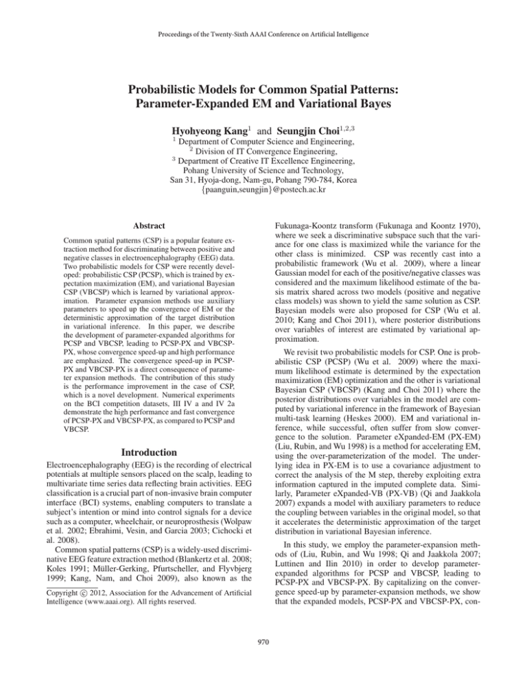
Proceedings of the Twenty-Sixth AAAI Conference on Artificial Intelligence
Probabilistic Models for Common Spatial Patterns:
Parameter-Expanded EM and Variational Bayes
Hyohyeong Kang1 and Seungjin Choi1,2,3
1
Department of Computer Science and Engineering,
2
Division of IT Convergence Engineering,
3
Department of Creative IT Excellence Engineering,
Pohang University of Science and Technology,
San 31, Hyoja-dong, Nam-gu, Pohang 790-784, Korea
{paanguin,seungjin}@postech.ac.kr
Abstract
Fukunaga-Koontz transform (Fukunaga and Koontz 1970),
where we seek a discriminative subspace such that the variance for one class is maximized while the variance for the
other class is minimized. CSP was recently cast into a
probabilistic framework (Wu et al. 2009), where a linear
Gaussian model for each of the positive/negative classes was
considered and the maximum likelihood estimate of the basis matrix shared across two models (positive and negative
class models) was shown to yield the same solution as CSP.
Bayesian models were also proposed for CSP (Wu et al.
2010; Kang and Choi 2011), where posterior distributions
over variables of interest are estimated by variational approximation.
Common spatial patterns (CSP) is a popular feature extraction method for discriminating between positive and
negative classes in electroencephalography (EEG) data.
Two probabilistic models for CSP were recently developed: probabilistic CSP (PCSP), which is trained by expectation maximization (EM), and variational Bayesian
CSP (VBCSP) which is learned by variational approximation. Parameter expansion methods use auxiliary
parameters to speed up the convergence of EM or the
deterministic approximation of the target distribution
in variational inference. In this paper, we describe
the development of parameter-expanded algorithms for
PCSP and VBCSP, leading to PCSP-PX and VBCSPPX, whose convergence speed-up and high performance
are emphasized. The convergence speed-up in PCSPPX and VBCSP-PX is a direct consequence of parameter expansion methods. The contribution of this study
is the performance improvement in the case of CSP,
which is a novel development. Numerical experiments
on the BCI competition datasets, III IV a and IV 2a
demonstrate the high performance and fast convergence
of PCSP-PX and VBCSP-PX, as compared to PCSP and
VBCSP.
We revisit two probabilistic models for CSP. One is probabilistic CSP (PCSP) (Wu et al. 2009) where the maximum likelihood estimate is determined by the expectation
maximization (EM) optimization and the other is variational
Bayesian CSP (VBCSP) (Kang and Choi 2011) where the
posterior distributions over variables in the model are computed by variational inference in the framework of Bayesian
multi-task learning (Heskes 2000). EM and variational inference, while successful, often suffer from slow convergence to the solution. Parameter eXpanded-EM (PX-EM)
(Liu, Rubin, and Wu 1998) is a method for accelerating EM,
using the over-parameterization of the model. The underlying idea in PX-EM is to use a covariance adjustment to
correct the analysis of the M step, thereby exploiting extra
information captured in the imputed complete data. Similarly, Parameter eXpanded-VB (PX-VB) (Qi and Jaakkola
2007) expands a model with auxiliary parameters to reduce
the coupling between variables in the original model, so that
it accelerates the deterministic approximation of the target
distribution in variational Bayesian inference.
Introduction
Electroencephalography (EEG) is the recording of electrical
potentials at multiple sensors placed on the scalp, leading to
multivariate time series data reflecting brain activities. EEG
classification is a crucial part of non-invasive brain computer
interface (BCI) systems, enabling computers to translate a
subject’s intention or mind into control signals for a device
such as a computer, wheelchair, or neuroprosthesis (Wolpaw
et al. 2002; Ebrahimi, Vesin, and Garcia 2003; Cichocki et
al. 2008).
Common spatial patterns (CSP) is a widely-used discriminative EEG feature extraction method (Blankertz et al. 2008;
Koles 1991; Müller-Gerking, Pfurtscheller, and Flyvbjerg
1999; Kang, Nam, and Choi 2009), also known as the
In this study, we employ the parameter-expansion methods of (Liu, Rubin, and Wu 1998; Qi and Jaakkola 2007;
Luttinen and Ilin 2010) in order to develop parameterexpanded algorithms for PCSP and VBCSP, leading to
PCSP-PX and VBCSP-PX. By capitalizing on the convergence speed-up by parameter-expansion methods, we show
that the expanded models, PCSP-PX and VBCSP-PX, con-
c 2012, Association for the Advancement of Artificial
Copyright Intelligence (www.aaai.org). All rights reserved.
970
(a) PCSP
(b) VBCSP
Figure 1: Graphical representation of PCSP and VBCSP models.
Gaussian distributions,
verge to solutions faster than PCSP and VBCSP. In addition,
we show that the generalization performance of PCSP-PX
and VBCSP-PX is better than that of PCSP and VBCSP.
In PCSP and VBCSP, feature vectors are constructed using only variances of the expected latent variables so that
the information on covariances is neglected. In contrast,
the auxiliary parameters in PCSP-PX and VBCSP-PX reduce such information loss by simultaneous diagonalization
of the second-order moments of the latent variables. This
is found to improve the generalization performance in the
classification. Numerical experiments on the BCI competition datasets, III IVa and IV 2a, confirmed that PCSP-PX and
VBCSP-PX not only speed-up the computations but also improve the classification performances of the feature vectors,
as compared to PCSP and VBCSP.
∼
(c)
∼
t
h
i−1 (c) ,
y t 0, Λ(c)
h
i−1 (c) ,
N t 0, Ψ(c)
(c)
yt
N
(c)
(c)
where Λ(c) = diag λ1 , . . . , λM ∈ RM ×M and Ψ(c) =
(c)
(c)
diag ψ1 , . . . , ψD ∈ RD×D are precision matrices for
c = 1, 2.
PCSP
In PCSP, the basis matrix A is treated as a matrix of pab ML
rameters, and their maximum likelihood estimate A
is determined by EM, where the E-step involves computing the expectation of the complete-data
log-likelihood
log p {X (c) }, {Y (c) } A, {Λ(c) }, {Ψ(c) } with respect to
the posterior distribution p {Y (c) } {X (c) } and the Mstep
A as well as other model parameters
n re-estimates
o
(c)
(c)
b −> is
Λ ,Ψ
. It was shown in (Wu et al. 2009) that A
Probabilistic Models for CSP
We briefly review two probabilistic models, PCSP (Wu et
al. 2009) and VBCSP (Kang and Choi 2011). The graphical
representations of these models are shown in Fig. 1(a) and
1(b), respectively.
Suppose that EEG signals involving two different mental
tasks (c ∈ {1, 2}) recorded at D electrodes over multiple tri(c)
als constitute a D-dimensional vector xt for t = 1, . . . , Tc ,
where Tc represents the number of samples obtained over
(c)
hmultiple trials.i We denote the EEG data matrix by X =
(c)
(c)
x1 , ..., xTc ∈ RD×Tc . The probabilistic model for CSP
ML
equal to the linear transformation matrix computed in CSP,
in the case of zero noise limit and when A is a square matrix. CSP feature vectors are constructed by taking logarithms of top-n variances of the projected variables for each
class within each trial. In the case of PCSP, CSP features are
computed using logarithms of top-n variances for each class
of posterior means over latent variables in each trial.
assumes that data matrices X (c) are generated by
VBCSP
X
(c)
= AY
(c)
+E
(c)
,
In VBCSP, the basis matrix A is treated as a matrix of random variables, and the automatic relevance determination
(ARD) prior is applied to it, i.e.,
(1)
where A = [a1 , . . . , aM ] ∈ RD×M is the basis matrix
shared across two classes (c = 1, 2),
h
(c)
(c)
p (A|D β ) =
i
Y (c) = y 1 , . . . , y Tc ∈ RM ×Tc ,
M
Y
−1
N [A]:,m |0, βm
ID ,
(2)
m=1
where I D ∈ RD×D is the identity matrix, D β ∈ RM ×M =
diag(β1 , . . . , βM ), and the precision hyperparameters βm
are assumed to follow Gamma distribution:
βm ∼ Gam aβ0 , bβ0 .
(3)
is the encoding
to latent variables),
h matrix (corresponding
i
(c)
(c)
and E (c) = 1 , . . . , Tc ∈ RD×Tc is the noise matrix.
Latent variables and noise are assumed to follow zero-mean
971
Inferring posterior distributions over βm leads us to predict
an appropriate number of columns in A. ARD priors are
(c)
(c)
also applied to {λm } and {ψd } (which are diagonal entries
of precision matrices Λ(c) and Ψ(c) ):
(c)
ψ ψ
λ λ
(4)
λ(c)
∼
Gam
a
,
b
,
ψ
∼
Gam
a
,
b
m
0 0
0
0 .
d
In the E-step, we compute the expected complete-data
log-likelihood hLc i
2 D
X
E
Θ ,
log p X (c) , Y (c)
∗
c=1
where the expectation h · i is taken with respect
to the posterior
distribution over latent variables
(c) (c) given the current estimate of paramp Y∗ X
n
o
eters Θ =
A∗ , Λ(c) , Ψ(c) , R . In the M-step, we
re-estimate parameters Θ that maximize hLc i computed
in the E-step. The EM iteration for PCSP-PX, which is
summarized in Algorithm 1, alternates between the E-step
and M-step until convergence.
In contrast to PCSP, the auxiliary parameters R should
also be optimized. The stationary point equation for R is
given by
!
2
2
D
E
X
X
∂ hLc i
(c)>
Tc R−> −
=
Λ(c) R Y (c)
Y
∗
∗
∂R
c=1
c=1
Variational posterior distributions are determined by variational Bayesian inference (Kang and Choi 2011). Again,
logarithms of top-n variances for each class of the variational posterior means of latent variables within each trial
are used as the CSP features.
Parameter-Expanded Algorithms
In this section, we present the main contribution of this
paper, parameter-expanded algorithms for both PCSP and
VBCSP. First, we introduce the parameter-expanded models (PCSP-PX and VBCSP-PX), as shown in Fig. 2(a) and
2(b), inspired by (Luttinen and Ilin 2010). Then we develop a parameter-expanded EM algorithm for PCSP-PX
and parameter-expanded variational Bayesian inference for
VBCSP-PX.
We introduce an invertible matrix R ∈ RM ×M . We de−1 (c)
fine A∗ = AR and Y (c)
Y . Then, we can write
∗ = R
the model (1) as
(c)
,
X (c) = A∗ Y (c)
∗ +E
=
0,
(6)
leading to
2
X
(5)
(c)
Λ
D
E
(c)>
R Y (c)
R> =
∗ Y∗
c=1
−1 (c)
Y . The invertible
for c = 1, 2, since A∗ Y (c)
∗ = ARR
matrix
R
introduces
a
transformation
of
the encoding man
o
trix Y (c) while preserving the conditional distribution
p X (c) A, Y (c) . We optimize the auxiliary parameters
R such that the expected complete-data log-likelihood (for
PCSP-PX) or the variational lower-bound (for VBCSP-PX)
is maximized.
2
X
!
Tc
IM ,
(7)
c=1
which is solved for R by simultaneous Ddiagonalization
E of
(1) (1)>
and
the second-order moments of encodings Y ∗ Y ∗
E
D
(2) (2)>
, followed by re-scaling.
Y∗ Y∗
The posterior distribution over latent variables in the original model is easily computed by
(c)
(c) (c) (c)
= N y t Rµt , RΣ(c) R> ,
p y t xt
PCSP-PX
(c)
where µt and Σ(c) are calculated in the E-step in Algorithm 1. We compute CSP features using posterior means
(c)
(c)
Rµt = RΣ(c) R> A> Ψ(c) xt that correspond to projected variables in CSP. Given test trial data X ∈ RD×T ,
we first compute T M -dimensional posterior mean vectors
over latent variables, constructing posterior mean matrices
(c)
Y
∈ RM ×T for c = 1, 2,
We present a parameter-expanded
EM o
algorithm to estimate
n
the model parameters A∗ , Λ(c) , Ψ(c) as well as auxiliary
parameters R. The basis matrix A in the original model
(1) is recovered by A∗ R−1 . To this end, we consider the
complete-data likelihood in the expanded model (5) (shown
in Fig. 2(a)):
o n
n
o
n
o n
o A∗ , Λ(c) , Ψ(c) , R
p X (c) , Y (c)
∗
Q2
(c)
(c) (c)
= c=1 p X (c) Y (c)
,
A
,
Ψ
p
Y
Λ
,
R
,
∗
∗
∗
Y
(c)
= RΣ(c) R> A> Ψ(c) X.
(c)
To model the project variables in CSP, we average Y
of
the two classes considering the class prior probability as
c
p(X ∈ (c)) = T1T+T
,
2
where
(c)
p X (c) Y (c)
,
A
,
Ψ
∗
∗
h
i−1 QTc
(c) (c)
= t=1
N xt A∗ y ∗t , Ψ(c)
,
(c)
p Y (c)
∗ Λ ,R
h
i−1 QTc
(c) > (c)
= t=1 N y ∗t 0, R Λ R
.
Y
=
2
X
c=1
Tc
(c)
Y .
T1 + T2
(8)
Then, we build a vector z ∈ RM , the m-th entry of which is
computed by
!
i
2
1h
1
>
[z]m = log
YY
−
Y 1T m
, (9)
T
T
m,m
972
(a) PCSP-PX
(b) VBCSP-PX
Figure 2: Graphical representation of PCSP-PX and VBCSP-PX models.
VBCSP-PX
Algorithm 1 EM for PCSP-PX
We present a parameter-expanded variational Bayesian
inference to speed up the deterministic approximation
of
over variables Z =
n the posterior distributions
o
(c)
(c)
Y (c)
,
A
,
β
,
Ψ
,
Λ
with
auxiliary parameters R.
∗
m
∗
(c)
Input: EEG data {X }.
Output: estimate of parameters Θ = {A∗ , Λ(c) , Ψ(c) , R}
initialize Θ = {A∗ , Λ(c) , Ψ(c) , R}.
repeat
E-step Calculate
the posterior
distribution over latent
(c) (c)
variables p y ∗t xt :
(c) (c)
(c) (c)
= N y ∗t µt , Σ(c) ,
p y ∗t xt
(c)
h
µt
i−1
Σ(c)
Variational posterior distributions over A and Y (c) in the
original model are easily recovered by variable transformation: A = A∗ R−1 n
and Y o(c) = RY (c)
∗ . We write the
(c)
joint distribution over X
and Z in the expanded model
(shown in Fig. 2(b)) with prior distributions defined in (2),
(3), and (4) as
n
o n
o
n
o n
o p X (c) , Y (c)
, A∗ , {βm } , Λ(c) , Ψ(c) R
∗
(c)
(c)
= Σ(c) A>
∗ Ψ xt ,
(c)
= R> Λ(c) R + A>
∗ Ψ A∗ .
M-step Re-estimate Θ:
- Update {A∗ , Λ(c) , Ψ(c) }:
=
2
Y
(c) (c)
Λ ,R
p Y (c)
p X (c) Y (c)
∗
∗ , A∗ , Ψ
c=1
[A∗ ]d,:
=
2
X
(c)
ψd [X (c) ]d,:
!
D
E
Y (c)>
∗
(c)
p Λ
M
Y
(c)
p Ψ
p(A∗ |D β , R)
p(βm ),
c=1
2
X
(c)
ψd
D
(c)>
Y (c)
∗ Y∗
!
E −1
m=1
where
Tc
h
i−1 Y
(c) > (c)
(c) (c)
N y ∗t 0, R Λ R
.
p Y ∗ Λ ,R =
,
c=1
h
(c)
ψd
i−1
h
i−1
λ(c)
m
=
=
D
E
1 h c (c)>
X X
− 2X (c) Y ∗(c)> A>
∗
Tc
D
E
i
(c)>
+A∗ Y (c)
A>
,
∗ Y∗
∗
d,d
1 h D (c) (c)> E > i
R Y∗ Y∗
R
.
Tc
m,m
t=1
The prior distribution over A∗ ∈ RD×M is assumed to be
matrix-variate Gaussian since it is not column-wise independent in contrast to (2). Thus we assume
p (A∗ |D β , R) = ND×M A∗ 0, I D ⊗ R> D −1
R
,
β
where matrix-variate Gaussian distribution for a random matrix B ∈ RD×M with mean matrix M ∈ RD×M and
covariance matrix ΩD ⊗ ΩM (ΩD ∈ RD×D and ΩM ∈
RM ×M ) takes the form
ND×M (B | M , ΩD ⊗ ΩM )
-D Solve (7) for
E R by
D simultaneous
E diagonalization of
(1)>
(2) (2)>
Y (1)
Y
and
Y
Y
to update R.
∗
∗
∗
∗
until convergence.
DM
M
D
(2π)− 2 |ΩD |− 2 |ΩM |− 2
1 −1
>
exp − tr Ω−1
(B
−
M
)Ω
(B
−
M
)
.
D
M
2
Note that the prior distribution over A in the original model,
given in (2), can also be written as
p (A|D β ) = ND×M A 0, I D ⊗ D −1
.
β
=
where 1T ∈ RT is the vector of all ones. We choose 2n
[z]m ’s with m corresponding to n largest and n smallest val(1)
(2)
ues of the ratio λm /λm to construct the CSP feature vector
2n
f ∈R .
973
Again, we can solve the equation for R by simultaneous
diagonalization
E moments of encodings
E of the
D second-order
D
(2) (2)>
(1) (1)>
, followed by re-scaling,
and Y ∗ Y ∗
Y∗ Y∗
as in PCSP-PX.
The variational inference involves the maximization of a
lower-bound on the marginal log-likelihood given by
n
o log p X (c) R
Z n
o
= log p X (c) , Z R dZ
n
o
Z
p X (c) , Z R
dZ
≥
q(Z) log
q(Z)
≡ F(q|R),
(10)
Algorithm 2 Variational Bayesian Inference for VBCSP-PX
Input: EEG data {X (c) }
Output: approximated posterior q(Z) for variables Z =
(c)
(c)
{A∗ , Y (c)
∗ , Λ , Ψ } and the auxiliary parameter R
initialize q(Z).
repeat
QD
- Update q(A∗ ) = d=1 N ([A∗ ]d,: |ν̄ d , Ωd ) by
where variational posterior distribution q(Z) is assumed to
factorize as
q(Z)
= q (A∗ ) q
−1
[Ωd ]
n
o
n
o n
o
(c)
(c)
(c)
y ∗t
q ({βm }) q ψd
q λm
.
Variational posterior distributions over each variable are alternatively updated such that the lower-bound F(q|R) is
maximized. Updating equations are summarized in Algorithm 2. In addition, auxiliary parameters R are optimized
by the maximization of F(q|R), given the variational posterior distribution q(Z). We consider the terms involving R
in the lower-bound F(q|R), given by
P2
c=1 Tc − D
log |R|2
2
2
E
D
E D
X
1
(c)>
R>
−
tr Λ(c) R Y (c)
∗ Y∗
2 c=1
D
E
1 −1
− tr hD β i R−> A>
A
R
.
(11)
∗
∗
2
Suppose aβ0 and bβ0 are set to small values so that hβm i can
be approximated as
hβm i =
'
aβm
bβm
=
bβ0 +
1
2
h
aβ0 + D/2
D
E
i
−1
R−> A>
∗ A∗ R
D
h
E
i
D
−1
R−> A>
∗ A∗ R
c=1
ν̄ d
=
h
D
c=1
m=1
c=1
0.
(c)
= N µt , Σ(c) by
h
i−1
Σ(c)
E
D
(c)
= R> Λ(c) R + A>
∗ Ψ A∗ ,
ED
E
D
(c)
(c)
Ψ(c) xt .
µt
= Σ(c) A>
∗
- Update q (βm ) = Gam aβm , bβm by
= aβ0 + D/2,
1 h −> D > E −1 i
bβm = bβ0 +
R
A∗ A∗ R
.
2
m,m
(c)
ψ(c) ψ(c)
- Update q ψd
= Gam ad , bd
by
aβm
m,m
ψ(c)
ad
ψ(c)
bd
m,m
= aψ
0 + Tc /2,
1 h (c) (c)>
X X
= bψ
+
0
2 D
E
−2 hA∗ i Y (c)
X (c)>
∗
D
Ei
(c)> >
+ A∗ Y (c)
Y
A
∗
∗
∗
E
i
.
d,d
(c)
λ(c) λ(c)
- Update q λm = Gam am , bm
by
m,m
(12)
aλ(c)
m
Applying the approximation (12) to (11), as in (Luttinen and
Ilin 2010), we have the stationary point equation for R given
by
∂F(q|R)
∂R
!
2
2 D
E D
E
X
X
(c)>
=
Tc − D R−> −
Λ(c) R Y (c)
Y
∗
∗
=
(c)
- Update q y ∗t
,
−1
hβm i R−> A>
∗ A∗ R
' M D.
2 D
E
D
E
X
(c)
=
ψd [X (c) ]d,: Y (c)>
Ωd .
∗
implying that
D
E
−1
tr hD β i R−> A>
∗ A∗ R
M
X
= R−1 hD β i R−>
2 D
E
ED
X
(c)
(c)>
+
,
ψd
Y (c)
∗ Y∗
bλ(c)
m
= aλ0 + Tc /2,
1 h D (c) (c)> E > i
= bλ0 +
R Y∗ Y∗
R
.
2
m,m
-DSolve (13) for
E R by
D simultaneous
E diagonalization of
(1)>
(2) (2)>
Y (1)
Y
and
Y
Y
to update R.
∗
∗
∗
∗
until convergence.
c=1
(13)
The approximated posterior over latent variables in the
974
original model is computed by
(c)
(c) q yt
= N y t Rµt , RΣ(c) R> ,
Compared to PCSP and VBCSP, parameter-expanded
algorithms PCSP-PX and VBCSP-PX perform additional
computation to optimize R at every iteration. However,
PCSP-PX and VBCSP-PX converge in a smaller number of
iterations; hence, they are faster than PCSP and VBCSP, respectively (Table 1). In general, the classification performance of PCSP-PX and VBCSP-PX was also higher than
that of PCSP and VBCSP (Fig. 3).
where µt and Σ(c) are calculated as in Algorithm 2.
We compute a CSP feature vector f for a test trial
(c)
X ∈ D RD×T
=
E the posterior means Rµt
E D using
(c)
(c)
>
(c)
xt ,
Ψ
A∗
RΣ
D
ED
E
(c)
Y
= RΣ(c) R> A> Ψ(c) X.
Conclusions
We have presented two new parameter-expanded algorithms
for PCSP and VBCSP, leading to PCSP-PX and VBCSPPX, where we expanded the models using auxiliary parameters R to speed up the convergence as well as to improve
the performance. The auxiliary parametersDR were estiE
(1)>
mated by simultaneous diagonalization of Y (1)
Y
∗
∗
D
E
(2) (2)>
and Y ∗ Y ∗
, reducing the coupling so that the convergence was accelerated and the performance was improved,
while CSP features determined by PCSP or VBCSP ignored
off-diagonal entries of the empirical second-order moment
matrix of posterior mean vectors. Numerical experiments
on the BCI competition datasets, III IVa and IV 2a, demonstrated the high performance of PCSP-PX and VBCSP-PX,
as compared to their counterparts PCSP and VBCSP.
We compute Y and [z]m as in (8) and (9). Then we select [z]m ’s with m corresponding
and n-smallest
D
E D to n-largest
E
(1)
(2)
values of the ratio of λm / λm to construct the CSP
feature vector f ∈ R2n .
Numerical Experiments
We compared the performances of PCSP, VBCSP, PCSPPX, and VBCSP-PX on the BCI competition datasets, III
IVa (Blankertz et al. 2006)1 and IV 2a 2 . Both datasets
consist of the EEG measurements of several subjects during
motor imagery tasks. The EEG data was pre-processed by
band-pass filtering, to emphasize important frequency bands
for recognizing the motor imagery tasks. Every trial was divided into the same number of time intervals after each visual cue, which contains EEG variation caused by the imagination of the subject.
We extracted feature vectors f ∈ R2n using PCSP,
VBCSP, PCSP-PX, and VBCSP-PX, and we applied the linear discriminant analysis (LDA) to transform these feature
vectors down to scalar values which are fed into a minimum
distance classifier. We set D = M and n = 3 for every
model. The classification performance of each model is represented by the prediction accuracy of the LDA classifier on
the test trials. The accuracy was calculated as the ratio of
the number of correctly classified trials to the total number
of test trials. We repeated the experiments 10 times, varying
the number of training trials, while the number of test trials
was fixed. We selected half of the trials in each data as the
test trials, and randomly selected some of the remaining trials as the training trials. The classes were strictly balanced
by selecting the same number of trials from each class.
BCI competition III IVa dataset was collected from five
subjects using 118 electrodes (D = 118) during the imagery movements of the right hand and right foot. The trials
were separated by up to 3.5s after each cue, and we used the
down-sampled version (100 Hz) of the data. 140 trials were
conducted for each subject and each class. BCI competition
IV 2a dataset contains 4 motor imagery tasks of 9 subjects,
recorded using 22 electrodes (D = 22). We considered only
the binary classification problem so that we selected the imagery left/right hand movement classes. The trials were separated by from 3.5s to 5.5s after each cue, and the sampling
rate was 250 Hz. 144 trials were conducted for each subject
and each class.
1
2
Acknowledgments: This work was supported by National Research Foundation (NRF) of Korea (2011-0018283,
2011-0018284), MEST Converging Research Center Program (2011K000673), NIPA Program of Software Engineering Technologies Development and Experts Education,
MKE and NIPA ”IT Consilience Creative Program” (C15151121-0003), and NRF World Class University Program
(R31-10100).
References
Blankertz, B.; Müller, K. R.; Krusierski, D. J.; Schalk,
G.; Wolpaw, J. R.; Schlögl, A.; Pfurtscheller, G.; and Birbaumer, N. 2006. The BCI competition III: Validating alternative approaches to actual BCI problems. IEEE Transactions on Neural Systems and Rehabilitation Engineering
14:153–159.
Blankertz, B.; Tomioka, R.; Lemm, S.; Kawanabe, M.; and
Müller, K. R. 2008. Optimizing spatial filters for robust
EEG single-trial analysis. IEEE Signal Processing Magazine 41–56.
Cichocki, A.; Washizawa, Y.; Rutkowski, T.; Bakardjian,
H.; Phan, A. H.; Choi, S.; Lee, H.; Zhao, Q.; Zhang, L.; and
Li, Y. 2008. Noninvasive BCIs: Multiway signal-processing
array decompositions. IEEE Computer 41(10):34–42.
Ebrahimi, T.; Vesin, J. F.; and Garcia, G. 2003. Braincomputer interface in multimedia communication. IEEE
Signal Processing Magazine 20(1):14–24.
Fukunaga, K., and Koontz, W. L. G. 1970. Application
of the Karhunen-Loève expansion to feature selection and
ordering. IEEE Transactions on Computers 19(4):311–318.
http://www.bbci.de/competition/iii/
http://www.bbci.de/competition/iv/
975
(a) III IVa data
(b) IV 2a data
Figure 3: Classification performances of existing methods (PCSP and VBCSP) as well as our proposed methods (PCSP-PX and
VBCSP-PX).
Table 1: Performance comparison in terms of number of iterations and run time. For each algorithm, the iterations stop when
the variant of the expected complete-data log-likelihood (for PCSP and PCSP-PX) or the variational lower-bound (for VBCSP
and VBCSP-PX) falls within a pre-defined value. The maximum number of iterations was set as 100 for each algorithm. The
’number of iterations’, ’run time’ and ’run time per iteration’ were averaged over multiple runs with 10 different training sets.
data
III IVa
IV 2a
measure
number of iterations
run time (sec)
run time per iteration
number of iterations
run time (sec)
run time per iteration
PCSP
86.6400 ± 24.0742
14.3137 ± 4.5311
0.1631 ± 0.0166
58.0417 ± 27.4807
0.1702 ± 0.0841
0.0029 ± 0.0003
PCSP-PX
15.7057 ± 7.0065
3.0026 ± 1.4251
0.1901 ± 0.0246
34.2093 ± 16.1989
0.1338 ± 0.0668
0.0039 ± 0.0004
Heskes, T. 2000. Empirical Bayes for learning to learn.
In Proceedings of the International Conference on Machine
Learning (ICML).
VBCSP
54.9114 ± 26.1892
37.1477 ± 16.7673
0.6917 ± 0.1013
18.5046 ± 7.9813
0.1579 ± 0.0740
0.0084 ± 0.0009
VBCSP-PX
13.8800 ± 3.4429
12.2370 ± 3.2140
0.8804 ± 0.0638
13.5111 ± 3.8341
0.1337 ± 0.0427
0.0098 ± 0.0011
classification in a movement task. Clinical Neurophysiology
110:787–798.
Qi, Y., and Jaakkola, T. S. 2007. Parameter expanded variational Bayeisian methods. In Advances in Neural Information Processing Systems (NIPS), volume 19. MIT Press.
Wolpaw, J. R.; Birbaumer, N.; McFarland, D. J.;
Pfurtscheller, G.; and Vaughan, T. M. 2002. Brain-computer
interfaces for communication and control. Clinical Neurophysiology 113:767–791.
Wu, W.; Chen, Z.; Gao, S.; and Brown, E. N. 2009. A
probabilistic framework for learning robust common spatial
patterns. In Proceedings of the 31st Annual International
Conference of the IEEE Engineering in Medicine and Biology Society.
Wu, W.; Chen, Z.; Gao, S.; and Brown, E. N. 2010. Hierarchical Bayesian modeling of inter-trial variability and variational Bayesian learning of common spatial patterns from
multichannel EEG. In Proceedings of the IEEE International Conference on Acoustics, Speech, and Signal Processing (ICASSP).
Kang, H., and Choi, S. 2011. Bayesian multi-task learning
for common spatial patterns. In Proceedings of the IEEE International Workshop on Pattern Recognition in NeuroImaging (PRNI).
Kang, H.; Nam, Y.; and Choi, S. 2009. Composite common
spatial pattern for subject-to-subject transfer. IEEE Signal
Processing Letters 16(8):683–686.
Koles, Z. J. 1991. The quantitative extraction and topographic mapping of the abnormal components. EEG and
Clinical Neurophysilology 79:440–447.
Liu, C.; Rubin, D. B.; and Wu, Y. N. 1998. Parameter expansion to accelerate EM: The PX-EM algorithm. Biometrika
85(4):755–770.
Luttinen, J., and Ilin, A. 2010. Transformations in variational Bayesian factor analysis to speed up learning. Neurocomputing 73:1093–1102.
Müller-Gerking, J.; Pfurtscheller, G.; and Flyvbjerg, H.
1999. Designing optimal spatial filters for single-trial EEG
976