Proceedings of the Twenty-Eighth AAAI Conference on Artificial Intelligence
Robust Visual Robot Localization Across Seasons Using Network Flows
Tayyab Naseer
University of Freiburg
naseer@cs.uni-freiburg.de
Luciano Spinello
Wolfram Burgard
University of Freiburg
spinello@cs.uni-freiburg.de
Cyrill Stachniss
University of Freiburg
University of Bonn
burgard@cs.uni-freiburg.de cyrill.stachniss@igg.uni-bonn.de
Abstract
Image-based localization is an important problem in
robotics and an integral part of visual mapping and navigation systems. An approach to robustly match images
to previously recorded ones must be able to cope with
seasonal changes especially when it is supposed to work
reliably over long periods of time. In this paper, we
present a novel approach to visual localization of mobile robots in outdoor environments, which is able to
deal with substantial seasonal changes. We formulate
image matching as a minimum cost flow problem in a
data association graph to effectively exploit sequence
information. This allows us to deal with non-matching
image sequences that result from temporal occlusions or
from visiting new places. We present extensive experimental evaluations under substantial seasonal changes.
Our approach achieves accurate matching across seasons and outperforms existing state-of-the-art methods
such as FABMAP2 and SeqSLAM.
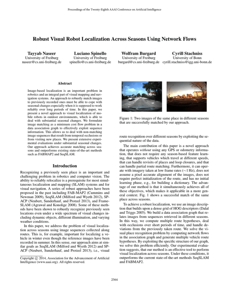
Figure 1: Two images of the same place in different seasons
that are successfully matched by our approach.
route recognition over different seasons by exploiting the sequential nature of the data.
The main contribution of this paper is a novel approach
that operates without using any GPS or odometry information, that does not require any season-based feature learning, that supports vehicles which travel at different speeds,
that can handle revisits of places and loop closures, and that
can handle partial route matching. Furthermore, it can operate with imagery taken at low frame rates (∼1 Hz), does not
assume a pixel accurate alignment of the images, does not
require perfect initialization of the route, and has no initial
learning phase, e.g., for building a dictionary. The advantage of our method is that it simultaneously achieves all of
these objectives, which makes it applicable in a more general context. Fig. 1 shows a successful match of the same
place across seasons.
To achieve a robust localization, we use an image description that builds upon a dense grid of HOG descriptors (Dalal
and Triggs 2005). We build a data association graph that relates images from sequences retrieved in different seasons.
In this way, we compute multiple route hypotheses, deal
with occlusions over short periods of time, and handle deviations from the previously taken route. We solve the visual place recognition problem by computing network flows
in the association graph and generate multiple vehicle route
hypotheses. By exploiting the specific structure of our graph,
we solve this problem efficiently. Our experimental evaluation suggests, that our method is an effective tool to perform
visual localization across seasons. Under these conditions, it
outperforms the current state-of-the-art methods SeqSLAM
and FABMAP2.
Introduction
Recognizing a previously seen place is an important and
challenging problem in robotics and computer vision. The
ability to reliably relocalize is a prerequisite for most simultaneous localization and mapping (SLAM) systems and for
visual navigation. A series of robust approaches have been
proposed in the past including FAB-MAP2 (Cummins and
Newman 2009), SeqSLAM (Milford and Wyeth 2012), SPACP (Neubert, Sunderhauf, and Protzel 2013), and FrameSLAM (Agrawal and Konolige 2008). Some of these methods have been shown to robustly recognize previously seen
locations even under a wide spectrum of visual changes including dynamic objects, different illumination, and varying
weather conditions.
In this paper, we address the problem of visual localization across seasons using image sequences collected along
routes. This is, for example, important for localizing a vehicle in winter even though the reference images have been
recorded in summer. In this sense, our approach aims at similar goals as SeqSLAM (Milford and Wyeth 2012) and SPACP (Neubert, Sunderhauf, and Protzel 2013), i.e., visual
c 2014, Association for the Advancement of Artificial
Copyright �
Intelligence (www.aaai.org). All rights reserved.
2564
Figure 2: Feature-based matching of the same place across
seasons. In this example, SURF features do not match reliably due to a substantial visual change.
Figure 3: Tessellation into cells for computing the image descriptor. A HOG feature is computed in each cell.
sumption of a linear velocity of the vehicle within each sequence. This assumption, however, is often violated in real
urban environments and robot applications. Neubert, Sunderhauf, and Protzel (2013) propose to combine an appearance change prediction with a vocabulary-based method to
predict how the visual word in the current scene would appear under changes. For learning the appearance changes
across seasons, an accurate image alignment is needed.
Johns and Yang (2013) learn discriminative statistics on the
co-occurrence of features over different conditions. This requires to learn stable and discriminative features over different times of the day or over different seasons. In our experiments, however, we were unable to obtain such stable and
discriminative features under the strong seasonal changes
that we experienced. Instead of explicitly addressing the visual place recognition with extreme perceptual differences,
Churchill and Newman (2012) associate different appearances, which they call as experiences, to the same place.
They localize in previously learnt experiences and associate
a new experience in case of a localization failure. At least
during the setup phase, this requires some degree of place
knowledge to assign a new experience to an existing place.
Our approach uses network flows to consider the sequential nature of the data in the individual routes. In other fields,
network flows have been successfully used to address data
association problems when tracking multiple people (Zhang,
Li, and Nevatia 2008; Ben Shitrit et al. 2013).
Related Work
Visual localization has a long history in computer vision and
robotics, see Fuentes-Pacheco, Ruiz-Ascencio, and RendónMancha (2012) for a recent survey. Large environmental and
seasonal variations are a major bottleneck towards robust
and long-term visual navigation. Various approaches have
been proposed to localize autonomous robots using visual
input (Cummins and Newman 2009; Davison et al. 2007;
Agrawal and Konolige 2008; Bennewitz et al. 2006). Visual localization with extreme perceptual variations has
been recognized as a major obstacle for persistent autonomous navigation and has been addressed by different researchers (Glover et al. 2010; Cummins and Newman 2009).
Biber and Duckett (2005) deal with changing indoor environments by sampling laser maps at multiple time scales.
Each sample of the map at a particular timescale is maintained and updated using the sensor data of the robot. This
allows them to model spatio-temporal variations in the map.
Stachniss and Burgard (2005), in contrast, aim at modeling different instances of typical states of the world using
a clustering approach. Many of the visual place recognition approaches rely on image matching by using features
such as SURF (Bay et al. 2008) and SIFT (Lowe 2004).
Such feature-based algorithms work reliably for matching
images that undergo rotation and scale variations but perform poor under extreme perceptual changes. Valgren and
Lilienthal (2010) made an attempt to use both features in
combination with geometric keypoint constraints for acrossseasons image matching. For our datasets, we found that
SIFT and SURF features do not match robustly, see Fig. 2
for an example. As a result, methods such as FAB-MAP2 by
Cummins and Newman (2009) that require a reliable matching of these features tend to fail. Furgale and Barfoot (2010)
propose a teach and repeat system for long term autonomy
using stereo vision. They create series of submaps during the
teach phase which relaxes the need of accurate global reconstruction while repeating the routes. Although, this approach
allows for navigating over longer routes, it does not address
large perceptual changes from the original traverse.
The goal of the work of Milford and Wyeth (2012), which
has a similar overall aim as our approach, is to match a sequence of query images to a sequence of database images.
The method computes a matching matrix which stores dissimilarity scores between all images in a query and database
sequence. The straight-line path through this matrix with the
minimum sum of dissimilarity scores across image pairs results in the best matched route. This corresponds to the as-
Visual Route Matching Across Seasons
We define the set D = (d1 , . . . , dD ) as the temporally ordered set of images that constitutes the visual map of places
(the database) and D = |D|. The set Q = (q1 , . . . , qQ ) with
Q = |Q| refers to the query sequence that was recorded in a
different season or after a substantial scene change.
Matching Images
Matching images of the same place between seasons is a
non-trivial task. The appearance of the same place is likely
to change substantially over the time of the year, see Fig. 1
for an example. Variations occur due to different weather
conditions, changing illumination, or other kinds of scene
change such as construction sites, new buildings, etc. In
most real world applications, re-visiting the same place typically happens under different conditions: the view-point of
the camera is not the same, the vehicle moves at different
speeds, and the framerate of the camera may differ. In particular, different seasonal weather conditions tend to have
2565
database images
notation:
query images
source
i,j
i,j
i+1,
j
i+1,
j
=
...
...
...
...
...
...
...
...
Figure 4: Illustration of the data association graph.
h d j · h qi
,
�hdj ��hqi �
...
i+1,
j+K
i+1,
j+K
...
...
Building the Data Association Flow Network
large impact on image-retrieval-based place recognition. For
example, during a snowy winter day, the landscape is covered by snow and the scene is poorly illuminated, yielding
few texture and low contrast. These settings cause images
to have weak gradients, which is suboptimal for computing
distinctive image descriptors. For this reason, place recognition methods that make use of keypoint-based feature detectors to compute region descriptors (Mikolajczyk et al. 2005)
are likely to detect only a small number of keypoints. The
scarcity of keypoints in turn yields only a limited number
of feature comparisons between images resulting in poor
matchings. Instead of relying on keypoints, we compute for
each image a fixed quantity of descriptors. To achieve this,
we tessellate the image into a grid of regular cells, see Fig. 3.
For each cell, we compute a HOG descriptor and combine
all descriptors into a single, dense description of the whole
image. The overall image descriptor h is a vector composed
of the concatenation of all the histograms of gradients computed on all the cells.
The resulting image descriptor is view-point dependent
due to the choice of the tessellation. To deal with this problem, we use large grid cells of 32 × 32 pixels in a 640x480
image. This decision is motivated by the particular choice
of HOG as grid feature. HOG describes a region by accumulating the gradient regardless to its location. As soon as
the same subject appears in the same cell, it is likely that
its descriptor is similar when the subject is seen from two
similar viewpoints. Moreover, the usage of HOG enables
matching under a range of different viewpoints and image
conditions (Dalal and Triggs 2005).
The distance between image qi ∈ Q and dj ∈ D is computed by the cosine distance of the two image descriptors,
respectively hqi and hdj :
=
i+1,
j+1
Figure 5: Illustration of the connections E a and E b between
matching (white) and hidden (red) nodes. The white rounded
rectangles are only used for illustration: an edge between
two rounded rectangles means that all nodes contained in
the first rectangle are connected via a directed edge to all
nodes in the second rectangle.
sink
cij
i+1,
j+1
A standard approach to image-based localization returns for
a query image in Q the best matching image in D according
to the matching matrix C. Due to the visual change across
seasons, a best-match-strategy in C typically results in a
poor localization performance. In this paper, we leverage
that Q and D consist of image sequences that are recorded
on a robot or vehicle. As a result, locations are visited progressively and images are not in random order. The matching
patterns in the matching matrix C reflect the temporal information of both sequences. Our approach exploits the sequential nature of data but does not assume that every image in Q
has a matching counterpart in D. We consider sequences that
can start and stop at any position in the query and database
set. Both sets might be composed of images that have been
recorded at different framerates or while traveling at different speeds.
In this paper, we propose to solve the visual route localization problem by building a flow network and computing its
minimum cost flow. The minimum cost flow problem consists of determining the most cost-effective way for sending
a fixed amount of flow through a network(Ahuja, Magnanti,
and Orlin 1993). The flow network is a directed graph with
at least one source node and one sink node. The source node
is the one that produces flow and the sink node is the one
that consumes flow. To each edge, we associate a cost w
and a capacity r. A source node is connected by only outgoing edges, a sink node by only ingoing edges. The capacity defines the number of units that can flow over an edge.
Our idea is to build a flow network to model the possible
matches between D and Q. A minimum cost flow algorithm
finds a set of paths that connect the source to the sink minimizing the path cost while transporting the specified flow
to the sink. Those paths represent multiple hypothesis about
the correct image matching and the estimation of the vehicle
route. In order to match complex temporal sequences that
include loops, we introduce special nodes to allow solutions
that include partially matched sequences.
In our approach, the network is a graph G = (X , E),
where X are the nodes and E the edges. We denote the quantity of flow generated by the source node as F ∈ N.
(1)
where cij ∈ [0, 1] and cij = 1 indicates a perfect match. The
matching matrix C has a size of Q × D and consists of all
cij , i.e., the cosine distances between all images of Q and
D, computed according to Eq. (1).
2566
Nodes The set X contains four types of nodes: the source
xs , the sink xt , the matching nodes xij , and so-called hidden nodes x̆ij . The node xs is the node that creates all the
flow F and xt is the only sink that consumes it. A node xij
represents a match between the i-th image in Q and the j-th
image D, i.e., that both images are from the same location.
There exists a hidden node x̆ij for each matching node xij .
The hidden nodes represent “non-matches” between images
and such nodes allow for paths even though the image pairs
cannot be matched. These nodes are traversed during short
temporal occlusions or non-matching sequences that occur
when the robot deviates from the original route.
value for typical city-like navigation scenarios. Edges connected to hidden states capture the fact that the corresponding images cannot be matched (due to strong changes, occlusions, etc.), but allow the path to continue through some
hidden nodes. The hidden nodes can also be used to terminate a matching sequence without terminating the overall localization process. This is important to handle situations in
which the vehicle temporarily deviates from the route taken
during mapping. Thanks to this graph design, G is a directed
acyclic graph (DAG).
Edge Costs and Capacity The cost of an edge connected
to a matching node xij is wij = c1ij , where cij is computed
in Eq. (1). In case that the edge is connected to an hidden
node, the weight is constant, w̆ = W . We determined this
parameter experimentally by using a precision-recall evaluation. In addition to that, we set the weight of the edges in
E s and E t to 0.
All edges that interconnect the hidden nodes have a capacity r = F + 1 so that they can be considered for usage
for each unit of flow. All the other edges have a capacity of
r = 1 so that they can be only used once. The path resulting
from the minimum cost flow on G corresponds to the best
data association between D and Q.
Edges The edges in G define the possible ways of traversing the graph from the source to the sink. Fig. 4 illustrates
the connectivity
of our�graph. We define four types of edges
�
in E = E s , E t , E a , E b The first set E s connects the source
to a matching node or to hidden node:
E s = {(xs , x1j ), (xs , x̆1j )}j=1,...,D
(2)
The set E s models that the first image of Q can be matched
with any image in the D via the matching nodes or that
no match is found via the hidden nodes. The second set of
edges, E t , represents all the connections that go to the sink:
�
�
(3)
E t = (xQj , xt ), (x̆Qj , xt ) j=1,...,D
Minimum Cost Flow For Vehicle Localization
In this section, we provide a probabilistic interpretation of
our solution for solving this problem. Without loss of generality, we present a formulation for F = 1. We define the
ordered set A = (xs , xa1 , . . . , xaA , xt ) where xai is a simplified notation indicating a vertex in X . The sequence A
is a route hypothesis, i.e., a sequence of matched images
between seasons. It contains only vertices that can be connected with the edges presented in the previous section. Each
sequence starts at the source and ends at the sink. For finding
the best matching visual route, we find the optimal sequence
A∗ with a maximum a posteriori approach:
The sink can be reached from any of the matching nodes
xQj and from the corresponding hidden nodes x̆Qj with j =
1, . . . , D. This models the matching or non-matching of the
last query image.
The set E a of edges establishes the connections between
the matching nodes as well as between the hidden nodes
�
�
E a = (xij , x(i+1)k ), (x̆ij , x̆(i+1)k ) i=1,...,Q,j=1,...,D, (4)
k=j,...,(j+K),k≤D
where k = j, . . . , (j + K). These edges allow for finding
sequences of matching images or sequences of unmatched
query images respectively. Finally, the last set E b of edges
connects hidden and matching nodes
�
�
E b = (xij , x̆(i+1)k ), (x̆ij , x(i+1)k ) i=1,...,Q,j=1,...,D, (5)
A∗ = argmax p (A | X )
A
= argmax p (X | A) p (A)
A
�
= argmax
p (xi | A) p (A)
k=j,...,(j+K),k≤D
The edges in E are the ones that are traversed when the sequence is not continued with the children of a node. Edges in
E b are the ones that are traversed when a matching is found
again so that the matching sequence can continue. See Fig. 5
for an illustration of the edges in E a and E b . As a design decision, there are no edges connecting nodes back in time,
mainly for constraining the search space. However, this is
not a limiting factor: loops in the route can be found by solving the flow network when F > 1.
The value of K specifies the number of considered path
hypotheses exiting from each node: the fan-out from a vertex defines which of the subsequent images can be concatenated to a path. Values for K > 1 allow for matching sequences recorded at different vehicle speeds or in case of
different camera framerates. An edge between nodes (i, j)
and (i+1, j) models a vehicle that does not move. In our implementation, we use K = 4, which seems to be a sufficient
b
A
(6)
i
We consider all the likelihood probabilities to be conditionally independent given A and define the prior p(A) as
p(A) = ps p(xa2 | xa1 ) . . . p(xaA | xaA−1 )pt
(7)
where ps and pt are the priors associated to the source and
sink. The term p(xai+1 | xai ) is proportional to cai+1 . We
define the likelihood p(xi | A) of xi being part of A as
�
1/Q if xi ∈ A
p(xi | A) =
(8)
0
otherwise.
To search for the best solution of Eq. (6), we use a minimum cost flow solver. An efficient implementation for minimum cost flow is the one �of Goldberg and�Kennedy (1995),
which has complexity O |X |2 |E| log |X | . In our context,
2567
0
0.8
200
Precision
Query (Summer)
100
1
Our method
Ground Truth
300
400
500
0.6
0.4
0.2
600
0
Figure 6: Two datasets visualized in a satellite image. The
vehicle route is shown in yellow.
200 400 600 800 10001200
Database (Winter)
0
0
Our method
SeqSLAM
HOG−bm
0.2
0.4 0.6
Recall
0.8
1
Figure 7: Left: Ground truth (thick) and our matching results (dots) . Right: Precision recall curve. Our approach accurately estimates the vehicle route and outperforms OpenSeqSLAM and the HOG-based best match strategy.
this is expensive as typical problems consist of hundreds or
thousands of images. Note that in the special case of F = 1,
finding a minimal cost flow is equivalent to find the shortest
path.
To solve this problem efficiently, we exploit the specific
structure of the graph. Our graph G is a DAG with nonnegative edges and each edge has either a capacity r = 1
or r = F + 1. This means that all paths through the matching nodes found by the minimum cost network flow consist in different paths. Given these restrictions, we formulate
an equivalent solution with a substantially smaller computational complexity. Computing a shortest path in a DAG
with a single source can be done by topological sorting in
O(|X | + |E|), which is even more efficient than Dijkstra’s
or the Bellman-Ford algorithm. Note that, in our case, |E|
depends linearly with respect to |X |. For depleting all flow
of the source node, we repeat this procedure F times. This
leads to an overall complexity of O(F |X |) = O(F Q D).
Each execution of the solver leads to a loop-free path of
the vehicle, as a consequence of our graph connectivity. The
flow F controls the maximum number of vehicle path hypotheses that are found in the graph. As there are at most F
iterations, the system returns the F best paths. In this way,
we are able to report sequences that include up to F traversals of the same loop. The parameter F is either set beforehand by limiting the search to F possible solutions or by
repeating the search until the computed path is dominated
by hidden nodes (non-matching events).
ing has been applied to the images.
Experimental Results
The first experiment is designed to illustrate that our method
is well-suited to perform matching across seasons. For this
experiment, we used a sequence of 676 summer and 1,322
winter images including labels corresponding to a track
length of around 3 km. The car drove approximately along
the same route but with different speeds and due to traffic, it
had to stop a few times at different locations while acquiring the query images. The sequence does not include any
loop and each query image has a matching counterpart in the
database. Fig. 1 shows a pair of images from this sequence.
The manually labeled ground truth matches in both sequences as well as our result are shown in the left image of
Fig. 7. For the evaluation, we accept a match if the resulting
true match is off by up to two images. We quantify the performance of our approach by using a precision-recall curve,
see the right image of Fig. 7. We compare against SeqSLAM, which is the current state of the art in cross-season
image matching, by using the OpenSeqSLAM implementation (Sunderhauf, Neubert, and Protzel 2013). The curve
“HOG-bm” refers to selecting the best match above a threshold using our tessellation-based HOG descriptor matching in
Eq. (1) without using the data association graph.
Our approach matches the summer and winter sequences
at a high degree of accuracy with precision and recall values
close to 1. It also successfully estimates the route of the vehicle even though the car was moving at different speeds
and stopped several times during the query run. Our approach is up to 3 times better in precision than OpenSeqSLAM and it reaches ∼0.95 Equal Error Rate (EER). The
Equal Error Rate is a measure of performance on precisionrecall graphs. OpenSeqSLAM achieves comparable precision results only at low recall rates. At increasing recall
rates, OpenSeqSLAM decreases in precision.
A second image sequence consists of 1,322 winter images (D) and 441 summer images (Q). This dataset is more
challenging as the matching sequence is interrupted and the
vehicle visited places in Q that have not been visited in D
and vice versa. Ground truth and our results as well as the
precision-recall curves are shown in Fig. 8.
Experimental Evaluation
Our evaluation shows that our approach accurately matches
image sequences across seasons and it outperforms two
state-of-the-art methods such as FABMAP2 and SeqSLAM.
For the evaluation, we recorded datasets by driving through
a city with a camera-equipped car during summer and winter. The datasets contain overlapping routes, typical acceleration and breaking maneuvers, other traffic participants,
variations in the camera pose, and seasonal as well as structural changes in the environment. Fig. 6 illustrates the circa
50 km long traveled path on a satellite map. The datasets
contain between 6,915 and 30,790 images. During summer,
we mounted the camera outside the car, whereas during winter we installed it behind the windshield. For evaluation, we
manually annotated a set of corresponding winter-summer
image pairs. No rectification, cropping, or other preprocess-
2568
1
200
300
0.6
0.4
0.2
400
0
200 400 600 800 10001200
Database (Winter)
Query (Summer)
0.8
100
0
0
Our method
SeqSLAM
HOG−bm
0.2
0.4 0.6
Recall
0.8
Query (Summer)
600
900
Our method
SeqSLAM
Ground Truth
0.6
0.4
0.2
200
400
Database (Winter)
0
0
Our method
SeqSLAM
HOG−bm
0.2
0.4 0.6
Recall
0.8
1
Figure 10: Left: Ground truth (thick) , our matching results
(dots), and OpenSeqSLAM (cross). Right: Precision recall
curve for the third dataset. Even though the query set contain
loops and places that are not in the database, our approach is
accurate and it outperforms SeqSLAM and the HOG-based
best match strategy .
Our approach again clearly outperforms OpenSeqSLAM.
It is up to 1.5 times better in precision than OpenSeqSLAM
and it reaches ∼0.82 EER. It also correctly estimates the
route of the vehicle even though not all query images match
the database. This means that the solution includes a path
through the data association graph that traverses hidden
nodes. From the hidden nodes, the path switched back to
matching nodes and continued to correctly match other images in the database.
Additionally, we compare our method to FABMAP2, another successful state-of-the-art method for place recognition. For the comparison to FABMAP2, we used the OpenFABMAP2 implementation by Glover et al. (2012). The
original binary version of FABMAP2 provided by the Oxford Mobile Robotics Group (Cummins and Newman 2009)
performs similar to OpenFABMAP2. For the sake of brevity,
results are reported only once. The results of OpenFABMAP2 are shown in Fig. 9. No meaningful matches are
found by OpenFABMAP2. We believe that may be caused
by the use of keypoint-based feature detectors in FABMAP2. As explained above, those may be suboptimal for
matching across seasons, e.g., see Fig. 2.
For the last experiment, we selected a database of 596
images from winter and 1,213 images from summer. This
dataset is the most challenging one as it contains loops
as well as places that the car never visited while building
D. Our approach is up to 2 times better in precision than
OpenSeqSLAM and it reaches ∼0.6 EER by using a flow
of F = 2 as shown in Fig. 10. This illustrates that our
approach is able to estimate the vehicle route even in the
case of place revisits and loops. At low recall-rates, our approach has lower accuracy but its advantage becomes clear
as soon as the recall-rate increases. In contrast to that, OpenSeqSLAM is not able to handle loops. In conclusion, our approach outperforms the state-of-the-art methods FABMAP2
and SeqSLAM.
Finally, our approach shows a comparable runtime to SeqSLAM. In all the experiments our approach takes between
2.1s and 3.7s on a regular PC using a single core.
Conclusions
We addressed the problem of visual localization by using
image sequences. We proposed a novel approach that is designed to perform localization even under substantial seasonal changes, e.g., summer vs. winter. We addressed the
problem by a HOG-based description of the images combined with a directed acyclic data association graph. We
formulated the problem of matching image sequences over
seasons as a minimum cost network flow problem and also
solved the issue of dealing with non-matching image sequences that may result from collecting data at new places.
Our experimental results suggest that our approach allows
for accurate and robust matching across seasons and that it
outperforms existing state-of-the-art methods such as FABMAP2 and SeqSLAM in this setting.
200
400
300
0.8
300
1200
0
1
Figure 8: Sequence in which the robot visits new places.
Left: Ground truth (thick) and our matching results (dots).
Right: Precision recall curve. Our approach outperforms
SeqSLAM and the HOG-based best match strategy in such
scenarios.
600
1
0
Precision
Our method
Ground Truth
Precision
Query (Summer)
0
Ground truth
OpenFABMAP
600
900
1200
Database (Winter)
Acknowledgements
Figure 9: OpenFABMAP2 results obtained by matching the
query images with the database without creating new places,
i.e., localization-only mode. Only few correct matches are
found by OpenFABMAP2. This is probably caused by using
SURF features for matching places across seasons.
This work has partly been supported by the European
Commission under FP7-ICT-600890-ROVINA, FP7-ICT610603-EUROPA2, and ERC-AG-PE7-267686-LIFENAV.
In addition to that, the authors would like to thank Noha
Radwan for her support during the experimental evaluation.
2569
References
ple times of day. In Proc. of the IEEE Int. Conf. on Robotics
and Automation (ICRA), 3507–3512.
Glover, A. J.; Maddern, W. P.; Warren, M.; Reid, S.; Milford,
M.; and Wyeth, G. 2012. Openfabmap: An open source toolbox for appearance-based loop closure detection. In Proc. of
the IEEE Int. Conf. on Robitics and Automation (ICRA).
Goldberg, A. V., and Kennedy, R. 1995. An efficient cost
scaling algorithm for the assignment problem. Mathematical
Programming 71(2):153–177.
Johns, E., and Yang, G.-Z. 2013. Feature co-occurrence
maps: Appearance-based localisation throughout the day. In
Proc. of the IEEE Int. Conf. on Robitics and Automation
(ICRA).
Lowe, D. 2004. Distinctive image features from scaleinvariant keypoints. Int. J. Comput. Vision 60(2):91–110.
Mikolajczyk, K.; Tuytelaars, T.; Schmid, C.; Zisserman, A.;
Matas, J.; Schaffalitzky, F.; Kadir, T.; and Gool, L. V. 2005.
A comparison of affine region detectors. Int. J. Comput.
Vision 65:2005.
Milford, M., and Wyeth, G. F. 2012. Seqslam: Visual routebased navigation for sunny summer days and stormy winter
nights. In Proc. of the IEEE Int. Conf. on Robitics and Automation (ICRA).
Neubert, P.; Sunderhauf, N.; and Protzel, P. 2013. Appearance change prediction for long-term navigation across
seasons. In Proc. of the European Conference on Mobile
Robotics (ECMR).
Stachniss, C., and Burgard, W. 2005. Mobile robot mapping and localization in non-static environments. In Proc. of
the National Conference on Artificial Intelligence (AAAI),
1324–1329.
Sunderhauf, N.; Neubert, P.; and Protzel, P. 2013. Are we
there yet? challenging seqslam on a 3000 km journey across
all four seasons. In Proc. of the ICRA Workshop on LongTerm Autonomy.
Valgren, C., and Lilienthal, A. 2010. SIFT, SURF &
Seasons: Appearance-based long-term localization in outdoor environments. Robotics and Autonomous Systems
85(2):149–156.
Zhang, L.; Li, Y.; and Nevatia, R. 2008. Global data association for multi-object tracking using network flows. In
Proc. of the IEEE Int. Conf. on Computer Vision and Pattern
Agrawal, M., and Konolige, K. 2008. Frameslam: From
bundle adjustment to real-time visual mapping. IEEE Transactions on Robotics 24(5).
Ahuja, R. K.; Magnanti, T. L.; and Orlin, J. B. 1993. Network flows: theory, algorithms, and applications. Prentice
hall.
Bay, H.; Ess, A.; Tuytelaars, T.; and Van Gool, L. 2008.
Speeded-up robust features (SURF). Comput. Vis. Image
Underst. 110(3):346–359.
Ben Shitrit, H.; Berclaz, J.; Fleuret, F.; and Fua, P. 2013.
Multi-commodity network flow for tracking multiple people. IEEE Trans. Pattern Anal. Mach. Intell. 99:1.
Bennewitz, M.; Stachniss, C.; Burgard, W.; and Behnke, S.
2006. Metric localization with scale-invariant visual features
using a single perspective camera. In European Robotics
Symposium, 143–157.
Biber, P., and Duckett, T. 2005. Dynamic maps for
long-term operation of mobile service robots. In Proc. of
Robotics: Science and Systems, 17–24. The MIT Press.
Churchill, W., and Newman, P. 2012. Practice makes perfect? managing and leveraging visual experiences for lifelong navigation. In Proc. of the IEEE Int. Conf. on Robitics
and Automation (ICRA).
Cummins, M., and Newman, P. 2009. Highly scalable
appearance-only SLAM - FAB-MAP 2.0. In Proc. of
Robotics: Science and Systems.
Dalal, N., and Triggs, B. 2005. Histograms of oriented gradients for human detection. In Proc. of the IEEE
Int. Conf. on Computer Vision and Pattern Recognition
(CVPR).
Davison, A. J.; Reid, I. D.; Molton, N. D.; and Stasse, O.
2007. Monoslam: Real-time single camera slam. IEEE
Trans. Pattern Anal. Mach. Intell. 29:2007.
Fuentes-Pacheco, J.; Ruiz-Ascencio, J.; and RendónMancha, J. 2012. Visual simultaneous localization and mapping: a survey. Artificial Intelligence Review 1–27.
Furgale, P. T., and Barfoot, T. D. 2010. Visual teach and
repeat for long-range rover autonomy. Int. J. Field Robotics
27:534–560.
Glover, A.; Maddern, W.; Milford, M.; and Wyeth, G. 2010.
FAB-MAP + RatSLAM: Appearance-based slam for multi-
2570